The production of this online material was supported by the ATRIUM European Union project, under Grant Agreement n. 101132163 and is part of the DARIAH-Campus platform for learning resources for the digital humanities.

Rasterization
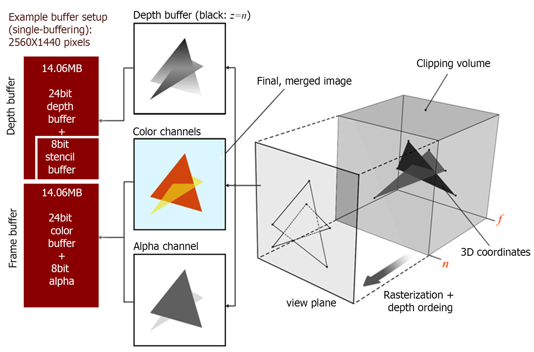
Rasterization is a primitive-order image synthesis architecture that processes a stream of primitives and converts them into a raster, i.e. an array of dense pixel samples, at the sampling rate of an image buffer. Each pixel sample is shaded individually and independently from all other pixels. The shaded pixel samples are then appropriately blended and combined with the already generated and stored samples in the image buffer to form the final image. A primary concern for image correctness in rasterization is the the elimination of hidden surfaces. The method is a primitive-order one in the sense that rendering is executed on primitives and each primitive is rasterized once per rendering pass, while the same image pixel location may be independently accessed for updates by multiple primitives overlapping in image space. Rasterization is fully implemented in hardware in all modern GPUs and is the mainstay for interactive rendering, due to its simplicity, efficiency, scalability and high performance.
The primary rasterization primitive is the triangle. Being convex by default, it greatly simplifies sample containment testing and therefore the rasterization process. Other important rasterization primitives are line segments and points. This small set of elementary primitives is adequate to sufficiently approximate other surfaces, since any polygonal surface can be constructed using triangles and linear segments can approximate any boundary curve.
The Rasterization Pipeline
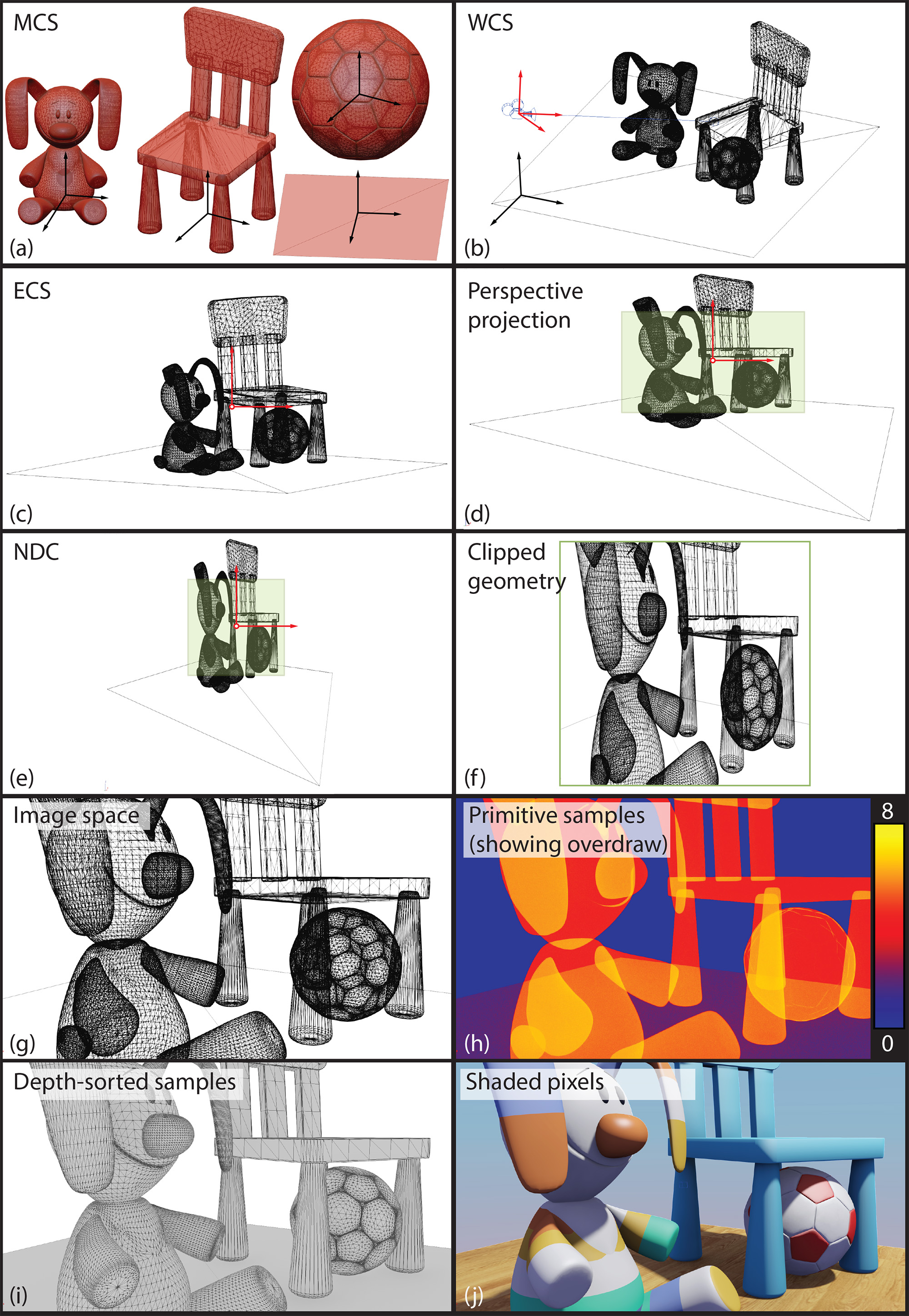
An overview of the rasterization pipeline is shown in the following figure. Primitive vertices are first transformed from the local (model) coordinate system of the object they belong to and then projected, obtaining their normalized device coordinates. Then the corresponding primitives are assembled and processed. Processing includes potential clipping and triangulation, tesselation, further vertex re-arrangement, primitive conversion or selective elimination.
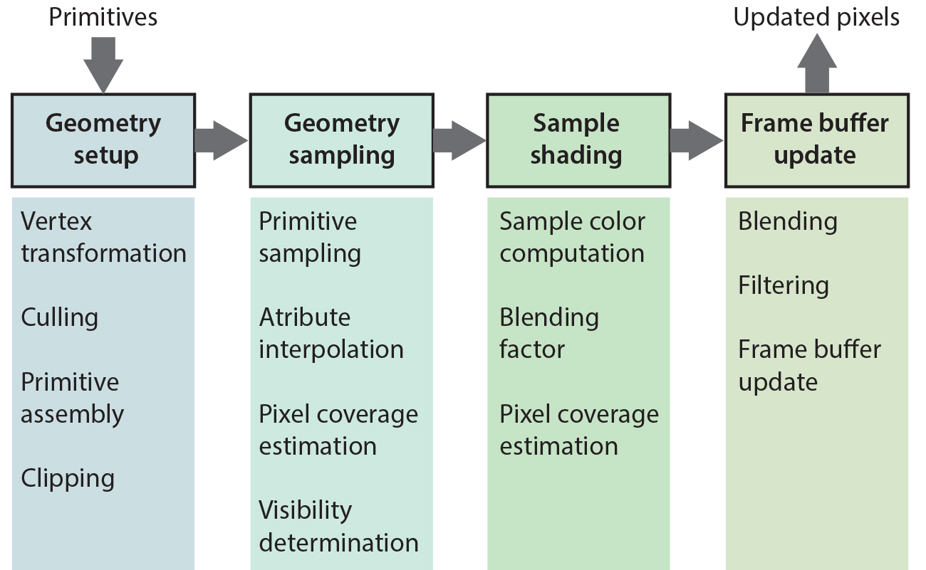
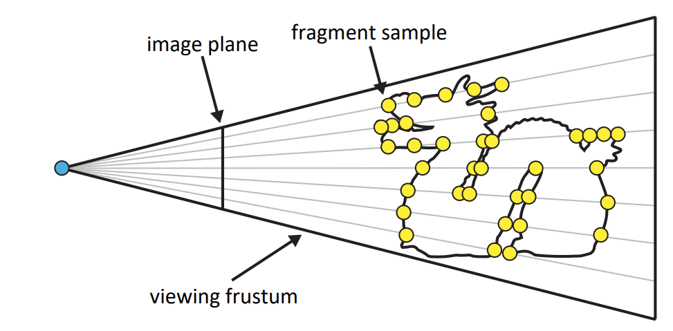
Next comes the dicing of a primitive into pixel-sized samples. These need to be efficiently determined (see below) and densely drawn, forming a contiguous region of pixels laid out on a grid within the boundaries of the rasterized primitive. For each generated primitive sample, the vertex attributes of the primitive are interpolated to obtain the corresponding values at the sample location. These are later used in the pixel shading operations for computing the color of the pixel sample. The pixel sample along with the record of interpolated attributes associated with it are often called a fragment1 to indicate that this is the smallest, indivisible piece of information that moves through the pipeline and to signify a potential decoupling between this token and the pixel, as sometimes the rasterization rate may differ from the final image buffer resolution.
A mandatory interpolated attribute that has a special significance for the rasterization pipeline is the sample’s normalized depth, i.e. its normalized distance from the center of projection. This value is used for the hidden surface elimination task, i.e. the determination of the visible samples and the discarding of any samples lying beyond the already computed parts of the geometry that cover a specific pixel. This test is typically performed as early as possible, i.e. after the sample’s depth has been determined, in order to reject non-visible samples as soon as possible. Depending on the specifics of the shading stage however, which may alter the state of the pixel sample, this test may be deferred to follow shading.
Since a primitive may not fully cover a pixel, being either too small or just partially intersecting the pixel, the pixel coverage may be optionally estimated, so that the assignment of the respective computed color to the frame buffer can be blended according to it, smoothly transitioning from the interior of the primitive to the "background" (see also antialiasing below).
After the sample generation, each record of per-pixel interpolated attributes is forwarded for shading, in a specific programmable stage, whose task is to compute the color of the current sample to be written to the designated output frame buffer. The allocation and specification of the output buffer in terms of format and dimensions is part of the pipeline setup. Please note that the frame buffer may correspond to the device’s output buffer to be accessed by the display terminal or an intermediate memory buffer allocated for the pipeline in GPU-addressable memory. Unless a plain color is output for a pixel sample, the fragment or pixel shading stage usually performs the most intensive computations, since it computes texturing and lighting to determine the output color. Additionally, this stage also calculates and assigns a "presence" value for the computed sample color, called the alpha value. This is typically used as a blending factor to mix the currently estimated pixel color with the color already present in the frame buffer, from the display of other primitives in the same pass. This is why the alpha value is involved in rasterizing surfaces with transparency 2.
The last stage of the simple forward rasterization pipeline is the deposition of the computed color for a given pixel onto the frame buffer either by substitution or blending of the underlying values. Blending adheres to specific rules that are governed by the blending function chosen and enabled, such as linear or additive blending. The alpha value of the new (source) fragment and optionally that of the existing (target) value are used as blending factors in this process. The GPU architecture handles the frame buffer update synchronization, to avoid conflicts when multiple triangles attempt to write at the same pixel location. Other clashes are avoided by explicitly generating a single sample per pixel per primitive.
The following figure presents a sequence of operations applied to the vertices of primitives, the primitives and the generated samples to form the final image.
Clipping
Clipping is a general computer graphics task that involves cutting out parts of one primitive against the outline of another and usually involves polygonal boundaries or linear segments. It is an important process for geometry processing and rendering as it allows computing intersections between primitives. In the case of the rasterization pipeline, we are interested in discarding parts of primitives that cross the boundaries of the view frustum and in particular the near clipping plane (see projections), since attributes interpolated for coordinates closer that the near clipping distance will be warped and in general, ill-defined. In principle, any clipping step we may perform on the near clipping plane we can repeat for the rest of the boundary planes of the frustum. However, it is more efficient to delay this until rasterization and perform the clipping in image space.
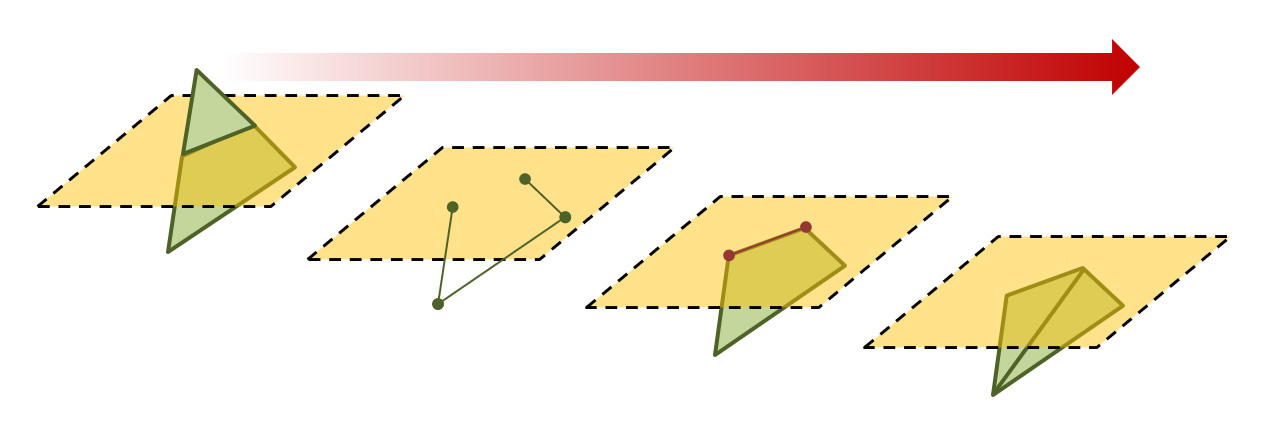
Clipping triangles in general results in convex polygons with more vertices. In the case of single-plane clipping (near plane), at most 6 vertices may be produced after clipping the triangular boundary by a quadrilateral viewport. Therefore, clipped triangles often need re-triangulation, which is trivial to implement for convex polygons, by constructing a fan-like collection of triangles to connect the vertices of the resulting boundary.
Sampling and Interpolation
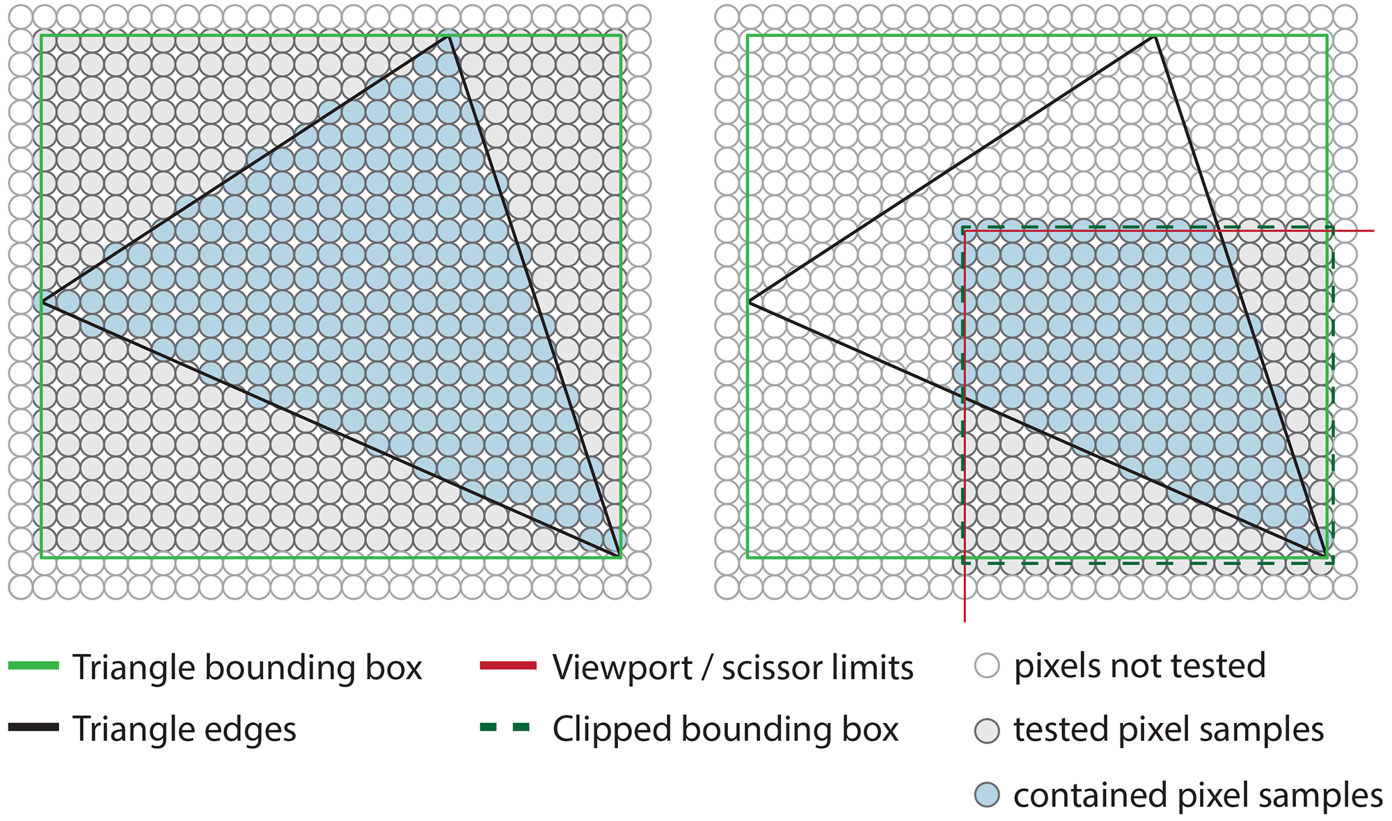
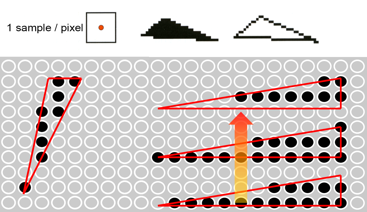
To compute the raster of a triangle, one needs to determine which pixels od the rendered image region are contained within the boundary of the triangle. First, the subset of potentially included pixels is determined, to avoid testing trivially external positions. One an do this by limiting the search for contained pixels to the intersection of the actual active rendering region and the horizontal and vertical extents of the triangle (see next figure - right). For each eligible candidate pixel, we test its relative position with respect to the three edges of the triangle, by means of an edge equation value, i.e. a specially constructed mathematical equation based on the coordinates of two consecutive triangle vertices, whose sign, when applied to the pixel’s coordinates, can determine which side of the boundary the pixel rests on. If the sign of this equation for a particular pixel is the same for all edges of the triangle, then the pixel is definitely inside the triangle and needs to be drawn. The calculation of the edge equations is very efficient, with most terms being computed once per triangle. Furthermore, the containment test can be trivially performed in parallel for all candidate pixels.
The geometric and textural properties for all interior pixels of triangle must be determined prior to forwarding these pixel samples for shading. Many user-defined properties may be uniform across the area of a triangle, e.g. a flat color, but typically, we need the attributes that we have assigned to the three vertices of the triangle interpolated inside its covered portion of the raster, to smoothly vary them across the triangle’s surface. There are also certain geometric aspects of the triangle that must be interpolated and especially the depth of the pixel sample, i.e. the third pixel coordinate (the other two being its image and coordinates).

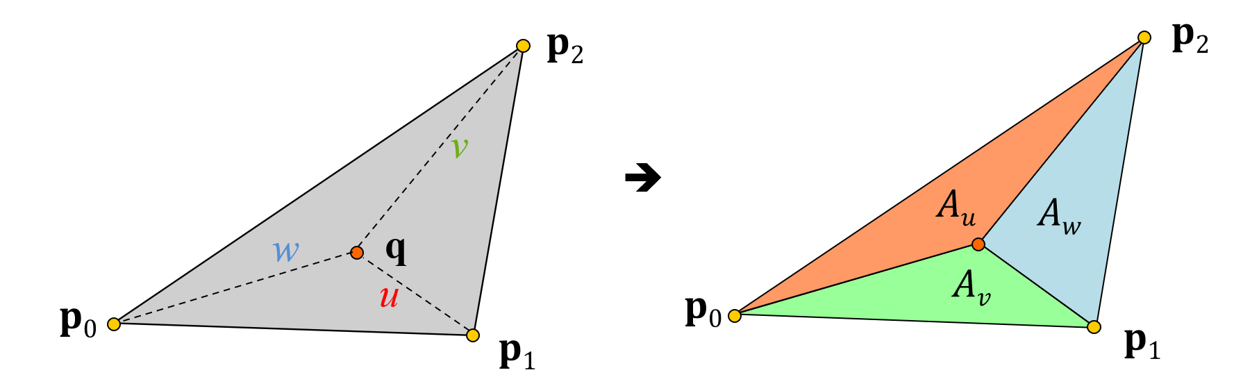
For each pixel that passes the containment test during rasterization, its attributes are interpolated and a fragment record is filled with the corresponding values. These will be later used for the shading of that pixel. The interpolation of the attributes itself is based on the three barycentric coordinates of the pixel’s position relative to the three vertices of the triangle (see figure below). The closer the pixel lies to a vertex, the larger is this vertex’s contribution to the linear blend of attributes that defines the interpolated values for the pixel. The barycentric coordinates are directly computed from the edge equation values for the point in question, with minimal extra overhead. The combined computation is very efficiently implemented in hardware and this is why the rasterization stage is quite fast.
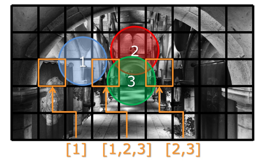
It is important to make a note here about a particular trait of rasterization that prevents it from being very efficient when rendering very small primitives. Pixel interpolation computations are done in pixel clusters and not for individual pixels. This is due to the fact that for shading computations that involve the determination of a mipmap level for one or more textures or certain calculations that involve image-domain attribute derivatives, the differences of the interpolated attributes with respect to neighboring pixels must be computed, even if these neighboring pixels are not part of the triangle interior. This is the case for boundary pixels and pixel-sized triangles. Therefore, it is more efficient to draw fewer large triangles, rather than many small ones. For the same reason, certain rasterization-based rendering engines have opted to handle the rendering of very small primitives with custom software implementations of rasterization rather than relying on the generic hardware rasterization units of a GPU3.
Hidden Surface Elimination
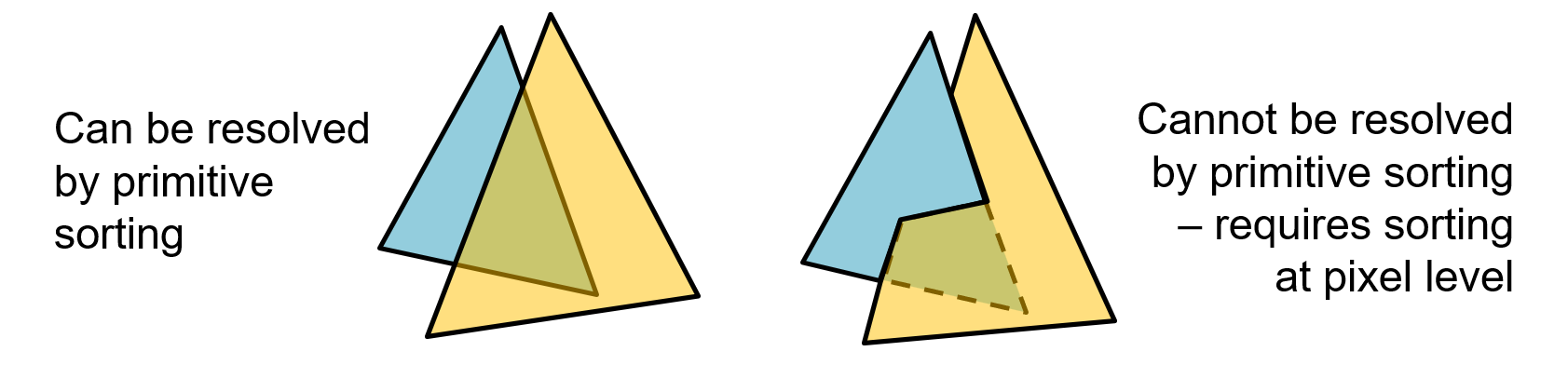
As explained in the introduction, in computer graphics, the task of hidden surface elimination is crucial for delivering a correct depiction of the order of presented surfaces and layers. Remember that in rasterization, all vertex coordinates have been first transformed to eye coordinates and then projected on the image plane. However, we cannot simply sort the triangles according to a layer or z-offset ordering, because this is an ill-defined problem; depth intervals of triangle edges may be overlapping and worse, triangles may just as well be intersecting each other, as shown in the next figure. Therefore, determining the closest, "visible" surface of a collection of triangles must be done at the smallest, atomic level of representation, i.e. the pixel. This is why, during the projection of a vertex on the image plane, its coordinate is not simply dropped, but is rather maintained either in its initial, linear form or in some other monotonic transformation, to be used for per-pixel depth comparisons in hidden surface elimination tests.
The easiest and most popular way to perform hidden surface elimination in the rasterization pipeline is the z-buffer algorithm. To implement the method, a special buffer, the depth buffer, equal in dimensions to the generated image is allocated and maintained, where the closest pixel depth values encountered so far during the generation of a single frame are stored. The depth values are typically normalized. At the beginning of each frame’s rendering pass, the depth buffer is cleared to the farthest possible value. For each interior triangle pixel sample generated by the rasterizer, its depth is compared to the existing value stored in the corresponding location in the depth buffer. IF the new sample’s depth is closer to the origin, the old depth value is replaced and the pixel sample is said to have "passed" the depth test; the sample’s fragment record is forwarded for shading. Otherwise, in the case of a failed depth test, the new sample is considered "hidden" and is discarded, undergoing no further processing.
Extending the mechanism of depth testing a little, the depth test itself can be changed from retaining the closest values to alternative comparisons, such as keeping the farthest or equidistant pixel samples, in order to manipulate the visual results and perform special rendering passes to implement specific algorithms and special effects. Furthermore, the depth buffer can be cleared to arbitrary values and the depth test can be completely switched off. This behavior is fully controlled by the application, which can set the appropriate rasterization pipeline state for the task at hand.
The depth test is triggered most of the time before shading, right after fragment interpolation, as it is prudent to avoid the expensive shading computations if the pixel sample is going to be eventually discarded as hidden behind other parts. However, there are certain rare shading operations that can unexpectedly alter the interpolated depth of a fragment and therefore, the depth cannot be relied upon for hidden surface elimination prior to shading. For these cases, the depth testing is performed after shading, introducing substantial overhead to the pipeline, since shading is performed for all generated pixel samples instead of only the visible ones.
Pixel Shading
The pixel coordinates inside a triangle marked for display are queued for shading. Since the rasterization pipeline enforces pixel independence, each primitive pixel sample is treated in isolation, meaning that it cannot access image-space information from neighboring image locations from the current image synthesis pass. However, we will discuss later on techniques that rely on multiple rendering passes, which enable the (re-)use of image-domain data at arbitrary pixels generated in previous stages to implement more complex shading algorithms.
In rasterization, shading involves the determination of a pixel sample’s color prior to updating the frame buffer and the determination of a presence factor, the alpha value, which is used for compositing the resulting color with the existing values in the same pixel location of the frame buffer. Shading alone is a common operation in all rendering pipelines, as shown in the appearance unit. However, the geometric and material attributes involved are computed differently in each pipeline and certain phenomena and light-matter interactions may not be possible to compute. Rasterization, relying on local geometric information alone, is incapable of estimating lighting contributions coming from other surfaces and therefore, in its basic form, it cannot compute indirect lighting, including reflections and proper refraction.
A typical single primitive rasterization pass that directly computes the shaded surface of primitives in the frame buffer, is called a forward rendering pass. The typical computations involved are the sampling of textures referenced by the geometry to obtain the local material attributes, the estimation of direct lighting from provided light sources, potentially involving light visibility (shadows). The alpha value of the shaded sample is also computed, but the particular stage does not control how it is going to be exploited by the rasterization pipeline. Furthermore, the shading algorithm my opt to completely discard the current fragment. This is particularly useful when attempting to render perforated geometry, where a texture layer provides an (alpha) mask for this purpose or the value is computed procedurally.
Optimizations
Since rasterization is a primitive-order projection-based approach to rendering, primitives not directly in view, play no part in the formation of the final image, at least for opaque objects. This means that if the visibility of entire clusters of primitives can be quickly determined prior to rasterization, these can be discarded early on, significantly reducing the processing load.
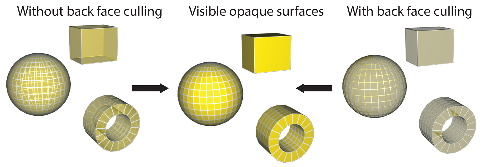
Back-face Culling
One of the easiest to test yet effective conditions for discarding geometry is back-face culling. It boils down to eliminating all polygons that are facing towards the front camera direction, i.e. they are showing their "back", or internal side to the view plane. The rationale behind this criterion is that at least for watertight objects, i.e. objects that are formed from closed surfaces with no gaps in the polygonal mesh, front-facing polygons should always be closer to the center of projection and therefore they should cover the back-facing ones anyway. Culling of the back-facing polygons is easily done by checking the sign of the coordinate of the geometric normal vector of the triangle’s plane, after projection, i.e. in clip space. The method is very efficient, eliminating on average 50% of the polygons to be displayed, regardless of viewing configuration. It is also orthogonal to other early culling techniques.
Keep in mind that the method is not generally applicable to transparent geometry, since the elimination of the back faces will be noticeable through the display of transparent front-facing polygons.
Hierarchical Depth Buffer
A hierarchical depth (Z) buffer (HiZ for short) organizes the depth buffer pixels in uniform blocks. Each block maintains the minimum and/or maximum depth values of the contained pixels and is updated each time a new fragment passes the depth test. This scheme can be recursively organized in more than two levels, by aggregating blocks in larger super-blocks. The hierarchical depth buffer can be used to accelerate various tasks, the most important being early fragment rejection: Since primitive fragments are (bi-)linearly interpolated, we can safely assume that, if the 4 corners of a block of fragments are contained within the boundaries of a primitive, we can check the minimum and maximum Z value and if outside the respective maximum and minimum values recorded as the block’s extents, the entire patch of fragments is rejected or accepted, without testing individual fragments. Another important use of the HiZ mechanism is the hierarchical screen-space ray marching that can be exploited for quickly skipping empty space when tracing rays in the image domain. Please read more on this, latter in this unit. higher levels of the HiZ construct are also utilized in occlusion culling, as they provide a "safer margin", a cheaper, low-resolution image space and a more cache-coherent way to query objects for visibility behind other, already drawn elements of a scene (see below).

Frustum culling
Since there is no indirect contribution of illumination coming from off-screen polygons to the generated image in rasterization, all geometry outside the view frustum can be eliminated right from the start. However, testing each and every polygon against the sides of the polyhedral clipping volume of the camera extents is not efficient, especially for large polygonal environments, negating the benefits of such an attempt. On the other hand, if we consider culling at the object level instead of the polygon one, far fewer tests are being executed per frame. For example, consider a forest consisting of 500 trees. Let us also assume an average polygon count of 10,000 triangles per tree. Attempting to draw the entire population of trees would result in emitting 5,000,000 triangles for rendering, which is very wasteful if the camera captures an angle from within or close to the forested area. attempting to cull this number of triangles is impractical, too. However, if we consider a simple bounding volume for each tree, such as its axes-aligned bounding box (AABB - see Geometry unit), then we only need to test 500 such simple primitives against the camera frustum, quickly eliminating thousands of triangles at once. This frustum culling optimization strategy occurs prior to submitting a workload of primitives for rendering and is generally orthogonal to back-face culling and per-primitive culling that follow.

Occlusion culling
Another technique for early culling of 3D objects in large environments is occlusion culling. In essence, it attempts to identify objects that are entirely hidden behind other geometry in the scene and flag them as invisible. For occlusion culling to make any practical sense, the cost of performing it must not outweigh the time saved by not rendering the eliminated geometry. This leads graphics engines to implement at least two or all of the following strategies when implementing occlusion culling:
Simplified testing. The bounding box of each one of the objects to be validated as hidden is typically considered and conservatively checked against a proxy of geometry already rendered so far (potential occluders). The current state of the partially complete depth buffer can serve as the occluder. Modern GPUs implement special queries (occlusion queries) for this type of testing, essentially counting the pixel samples that survive the depth test.
Temporal reuse. Provided a smooth frame rate can be maintained, the visibility does not change significantly from frame to frame. This provides ample opportunity for reuse of visibility results, lazy re-evaluation and out-of-order scheduling of visibility and rendering passes. To account for fast moving objects, their bounding volumes may also be dynamically enlarged (compensating for the motion vectors) to ensure conservative occlusion queries. One way to exploit this is to use a version of the depth buffer from the previous frame, reprojected to compensate for the camera motion between frames. Another viable option is to use as occluder a quickly prepared depth buffer of the objects that were marked as visible in the previous buffer, in a pre-pass in the current frame.
Hierarchical testing. Bounding volume hierarchies (see Geometry unit) can be exploited instead of a flat set of object bounding volumes, to both cull aggregations of objects with a single operation and quickly update visibility query results up and down the hierarchy of "occludees" (bounding volumes)4.
State change minimization
A useful optimization that is orthogonal to other approaches is the minimization of graphics state changes. When emitting a work queue for processing (rendering) to the GPU, a large set of parameters must be configured, variables need to be updated, executable code has to be loaded and made ready to run and internal buffer memory has to be allocated. All these steps configure a rasterization pipeline to run in a specific way and generate a desired rendered appearance for the emitted primitives. On the other hand, chunks of geometry from the virtual environment typically have different material attributes and some times require different geometry manipulation and shading algorithms to run on the GPU to display them. For example, certain parts of the environment may be rendered as wireframe outlines, others may require solid shading or transparent rendering. Off-screen computations involving shadow generation, environment lighting or other rendering passes may also need to be prepared prior to rendering parts of the environment. All these different configurations also represent significant changes to the setup of the rendering pipeline. Arbitrarily and repeatedly modifying the graphics state whenever a particular draw call requires some change is not ideal, as it introduces significant overhead. It is therefore prudent to pre-sort the draw calls (and respective parts of the scene) according to state and avoid constant state switching. For instance, sorting renderable elements according to the shader used (see next) is a good idea. This optimization can be intuitively implemented in an entity component system5, a software architecture for developing game- and graphics-oriented platforms. Entities, i.e. objects to be (potentially) rendered may have different components, each one associated with the object’s characteristics (e.g. shadow caster, glowing, transparent), while a system, i.e. here a rendering pass requiring a specific graphics state, scans over all entities and triggers a rendering call only for those that have a compatible component attached.
Shaders
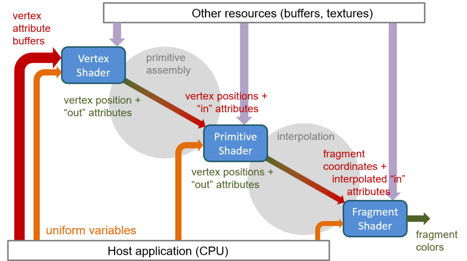
The vertex, primitive processing and pixel shading stages are to a large extent programmable, allowing custom transformations and arbitrary vertex attributes to be computed and forwarded down the pipeline. Primitives can also be procedurally reconfigured or refined. In the programmable stages of the pipeline, shaders are executed to perform the various computations. These shaders are functions (potentially invoking other functions in their turn) with a well-defined input and output, which are written in special human-readable programming languages called shading languages, compiled into native GPU machine code by the driver’s shader compiler and linked together to form a cascade of inter-operating stages that define the specific function of the rendering pipeline.
As expected, all programmable stages of the pipeline may request random access to read resources that are potentially required by the code being executed to perform the computation. Such resources are typically image buffers that represent material textures, pre-computed data or frame buffer information produced by previous rendering cycles. Randomly accessing memory buffers for writing is also possible but not always efficient, due to the need to ensure exclusive access to memory locations during the parallel execution of the code in the GPU cores. The following simplified diagram illustrates this idea.
Shader Types
First, the pipeline is set up to work with specific pieces of machine code (the compiled shaders) that have been linked into a unified pipeline of programmable stages, the shader program. In each subsequent call to draw a set of geometric primitives (line segments, polygons, points), the attributes of each primitive vertex are passed to the vertex shader. Along with the vertex attributes, the vertex shader also has access to a number of variables, which are set by the host system and are considered immutable during a rendering call to draw a set of elements and accessible by all programmable stages. They are called uniform variables due to the particular expectation (and implemented data synchronization policy) that they cannot change between individual calls to draw elements. Uniform variables are very important for the entire shading pipeline, as they pass global variables necessary for the calculations in the programmable stages, such as geometric transformation matrices, material parameters, textures and illumination properties. In essence, every piece of information that is not part of a vertex attribute record, has to be passed to the programmable rasterization pipeline via a uniform variable in order for a shader to have access to it. The primary task of a vertex shader is to transform geometric data such as positions (mandatory) and normal or other vectors defined in local coordinates of the rendered elements to clip (normalized post-projective) space. A vertex shader optionally computes other vertex data, e.g. the position in other coordinate systems, such as ECS or WCS and repack or expand other attributes, such as vertex color information and texture coordinates.
An optional general stage that follows the vertex shader is what we call here a "primitive shader". This, depending on the specific implementation of the rasterization pipeline, can take many manifestations, from the generic geometry shader stage, to the more specific ones. such as the tesselation and mesh shaders, some of which are vendor-specific. The common underlying property in this family of shaders is that they operate on primitives, as a cluster of vertex and connectivity information, not on isolated vertices. This is useful for augmenting the primitive, e.g. subdividing — "dicing" — it into more, smaller primitives to produce finer and smoother details, replacing the geometric element type (e.g. build polygons out of point primitives to efficiently construct particles), or discarding and redirecting primitives to specific rasterization "layers".
The final mandatory stage is the fragment or pixel shader, which processes the records of the sampled points on the primitive, as these have been interpolated by the rasterizer, to produce the color, alpha value and other, complementary data to the output frame buffer(s). Typically, a single RGB+A frame buffer is allocated and bound to the output of the pipeline for pixel value writes, but this buffer representation can be extended to support more than 4 channels, by concatenating multiple rendering targets, i.e. allocated RGBA frame buffer attachments. Additionally, shaders can perform updates to random-access memory buffers resident on the GPU, but usually, specific synchronization is required to avoid overlapping the updates during parallel shader code execution. Conversely, when writing to the conventional fragment shader output frame buffer, race conditions can be more efficiently handled, since for any primitive, the generated fragments are non-overlapping in image space and primitive processing order is maintained. The primary role of the fragment shader is to compute the output color of the currently shaded pixel location. This computation can be anything from a a simple solid color assignment to complex illumination and texturing effects (see appearance unit). In this respect, it is expected that the particular shader is generally the most computationally intensive, both in terms of calculations and resource access requests (texture maps).
A Simple Shader Program
In the following two snippets of code, we present an example of a simple vertex and an even simpler fragment shader.
Let us break down the two pieces of code, written in the Open GL Shading Language (GLSL), a common shader code definition language. The vertex shader first declares the attribute binding, by stating that the first vertex attribute passed (location 0) is assumed to be the vertex position coordinates, hereafter referred to by the variable name "position" and the second attribute (location 1) is the normal vector coordinates. Both variables are three-coordinate vectors (x,y,z). Next, the shader declares that it is expecting the binding of 3 uniform variables with the specific names provided in the code, all representing and storing transformation matrix data: the geometric transformation that expresses the object-space position coordinates of the vertex in the eye (camera) coordinate system, the projection matrix that projects points to the plane and transforms them to clip space coordinates and finally, a transformation matrix for expressing directions (the normal vectors here) from object space to eye coordinates. The surface normals are passed along as input to the vertex shader and are required for shading computations in the fragment shader. The particular calculation, computes a shading value by comparing the normal vector with the camera viewing direction. If the normal vector is converted to eye coordinates, the computation is simplified and no additional "viewing direction" uniform variables need to be passed to the fragment shader. Here, for the shading that follows, we have also declared an additional output vector, n_ecs, which will carry over the result of the transformed normal vector to the interpolator and then to the pixel samples, for shading. The only function present in this particular vertex shader is the mandatory "main" function, which has a compulsory output, the gl_Position, corresponding to the clip space coordinates of the processed vertex. The vertex shader function computes the two output vectors (clip space position and eye space normal) by applying the appropriate sequence of transformation matrices and doing the necessary vector conversions.
// Vertex shader.
#version 330 core

// vertex attributes used by the vertex shader.
layout(location = 0) in vec3 position;
layout(location = 1) in vec3 normal;

// uniform variables accessed by the shader.
uniform mat4 M_obj2ecs;   // "modelview" matrix: local object space
                          // coordinates to eye coordinates transformation

uniform mat4 M_proj;      // projection matrix

uniform mat3 M_normals;   // inverse transpose of the upper-left 3x3 of the
                          // modelview matrix

out vec3 n_ecs;           // optional output of the vertex shader:
                          // Normal vector in ECS coordinates.

void main()
{
	// compulsory output: the normalized clip-space coordinates of the
	// vertex position
	gl_Position = M_proj * M_obj2ecs * vec4(position, 1.0);

	// eye-space (camera) coordinates of the normal vector.
	n_ecs = M_normals * normal;
}
// Fragment shader.
#version 330 core
// Optional sampled attributes
in vec3 n_ecs; // the interpolated normal vector computed in the
// vertex shader.
out vec4 frag_color; // The shader output variable (RGBA)
void main()
{
// Simple shading: maximum lighting when normal faces the camera (+Z)
vec3 n = normalize(n_ecs); // Interpolated normals are no more of
// unit length. Must normalize them.
// Simple diffuse shading with virtual directional light
// coming from the camera. Assume a red surface color: (1,0,0)
vec3 color = vec3(1.0, 0.0, 0.0);
float diffuse = max(n.z, 0.0);
frag_color = vec4(color*diffuse, 1.0);
}In the fragment shader of this example, where the pixel sample records end up after interpolation of the primitive attributes by the rasterizer, there are a number of compulsory input data that are passed, including the fragment coordinates. The user-defined additional output of the vertex shader is interpolated along with the mandatory attributes and declared here as input (in vec3 n_ecs). In the main function (the only function in this code), the normal vector is first normalized, since linear interpolation does not retain the unit length of the shading normal, if different at each vertex. Then, the shading is computed by assuming a light source positioned directly at the camera: We take the dot product between the normal vector and the eye direction (positive Z axis in eye space coordinates). This corresponds to the cosine of the angle between two directions and translates to diffuse shading radiance flow. Fortunately, in this case, since we have converted the normal vector to eye space coordinates in the vertex shader, the dot product is simplified, since = = . To avoid negative values for flipped polygons, the shading is also clamped to zero. Finally, the output color is the shading coefficient multiplied by the base color of the surface (here we do not use a physically-correct model). The alpha value of the output fragment is always 1.0 in this example, signifying an opaque primitive or, more generally, one with maximum blending presence.
Antialiasing
During the rasterization step, where image samples are drawn and a decision is taken regarding the inclusion of this sample or not inthe set of pixel samples to be forwarded for shading, this decision is so far binary: The pixel sample is either retained, as belonging to the primitive, or rejected, as not being part of the primitive. Yet, this decision is based on a particular sampling of the image raster with a specific (fixed) sampling rate, dependent on the image resolution. For samples at the boundary between the "interior"6 of the primitive and the background, this binary decision introduces aliasing, since there is no practical frequency that can effectively sample and reconstruct an abrupt transition from the interior to the exterior of the primitive. In practical terms, we can never display a primitive correctly, in the strict, mathematical sense, unless its border is either vertical or horizontal and exactly coincides with the midpoint between two columns or rows of pixels, respectively. We can only approximate its shape with a varying degree of success. Now going back to our one-sample-per pixel rasterization mechanism, turning a pixel on or off for a primitive with full or no pixel coverage, respectively, invariably creates a pixelized look to the rendered primitives. Worse, for thin structures, entire primitives may be under-sampled or even completely missed.
Since we cannot raise the sampling rate of our image beyond what the target resolution can offer, we have to resolve to various band-limiting (low-pass filtering) techniques to "smooth" the rendered primitives. The prevailing techniques in computer graphics are all in the post-filtering domain, using multiple samples at a higher spatio-temporal rate and then averaging the result to conform with the particular single frame resolution. This does not mean that there are no pre-filtering methods in the literature, but they tend to be too specialized to be practical. We present below some of the most common types of antialiasing techniques.
Super-sampling (SSAA)
Supersampling can be considered a brute-force way to mitigate the insufficient resolution of the raster grid, but in no way can it solve the aliasing problem. In essence, it allows to extend the native sampling rate to correctly capture higher frequencies and then subject the resulting signal to a low-pass filter operator to adjust the signal to the maximum attainable frequency of the actual image. In other words, yes, supersampling can improve the fidelity of the image, by smoothing transitions and more accurately representing sub-pixel features, but practically only mitigates the problem to even smaller details. The most important drawback of supersampling comes from the fact that it literally multiplies the actual samples taken on the raster plane, increasing the number of containment tests and shading operations proportionally to the oversampling rate. For instance, quadrupling the number of image samples (4 samples per pixel), results in 4 points being tested for containment and the resulting active samples being all shaded. The resulting shading values are then averaged. Keep in mind that in the case that not all pixel samples are validly contained within the primitive’s effective area, the coverage of the pixel is not 100%. Instead, the ratio of the contained sub-pixel samples over the total sub-pixel samples are considered as the "presence" of the pixel, establishing the amount of partial occupation of the pixel by the primitive. This factor is used to properly blend border pixels with the contents of the frame buffer.
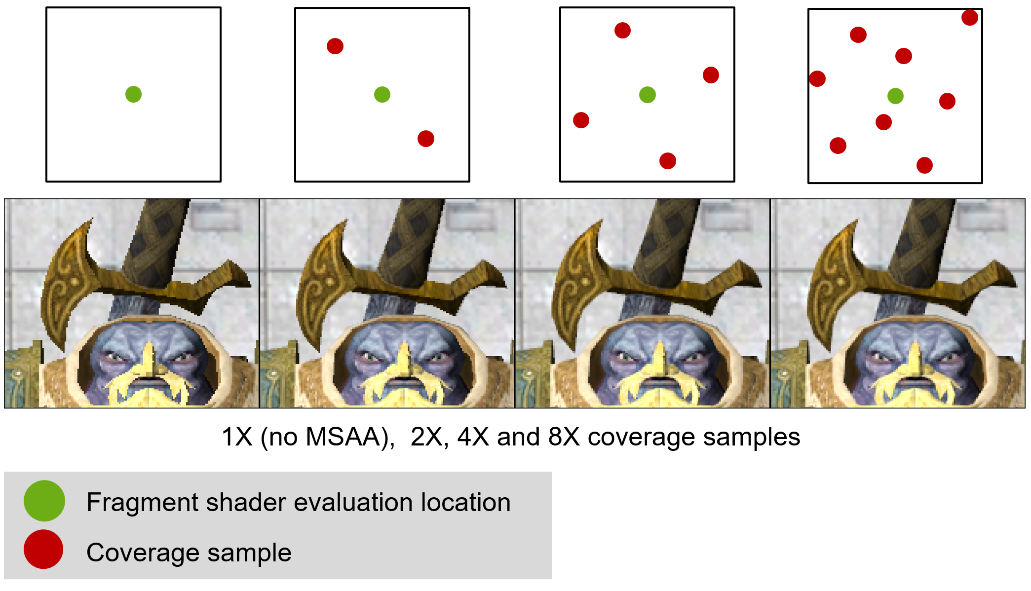
Multi-sampled Antialiasing (MSAA)
Although SSAA is quite effective in smoothing the image, it is also very expensive, since the shading computations are multiplied by (up to7) the super-sampling factor. To avoid the overhead, a trade-off has been devised: instead of evaluating shading for all sub-pixel samples, a single sample is used for shading computation and the rest are only used for determining the pixel coverage. The pixel coverage only involves the primitive containment testing method, which is very fast to evaluate by the rasterizer, while the cost of shading is the same as not performing antialiasing at all. This technique, which has been implemented in GPU hardware from simple mobile GPUs to desktop ones, is called multi-sampled antialiasing (MSAA) to differentiate the approach from the brute-force SSAA. However, MSAA trades accuracy for speed since: a) it only evaluates 1 sample, inheriting any shading-induced aliasing artifacts, such as shadow determination artifacts and specular "fireflies" and b) the exact point to use for shading may not be representative of the cluster of the coverage samples. It is possible to determine a good shading evaluation position (e.g. the cover sub-pixel samples average location), but with some additional cost.
Temporal Antialiasing (TAA)
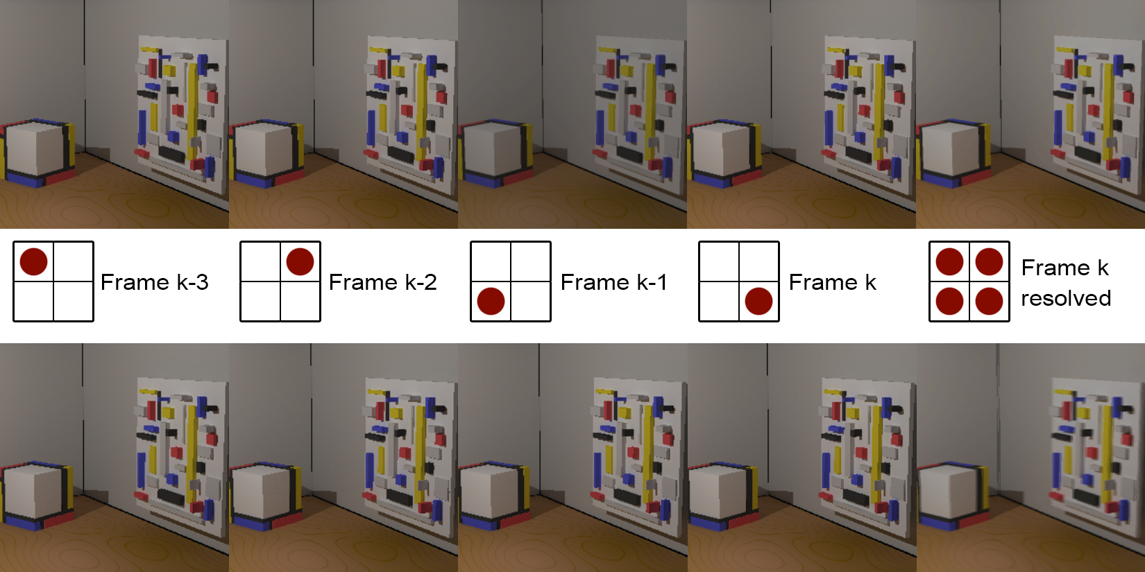
Temporal antialiasing is a special form of super-sampled antialiasing that instead of only spatially distributing the samples over the pixel area, in instead uses a spatio-temporal distribution, spreading samples across time by using sample positions from previous frames to amortize the cost of computing all sub-pixel samples (and shading) for a pixel in the same frame. To resolve the antialiased image in frame , the frame buffer contents of the previous frames are also re-used. In a simple implementation, as shown in the following figure (with ), a different sub-pixel sampling location is used in every frame, which can by repeated every frames. allocated buffers are used, averaging the current frame with the previous frames to obtain a resolved antialiased image. The accumulated values of previously generated frames can also be used instead in a running average with an exponential decay, to save frame buffer memory. This simple technique is valid and effective if the contents of the image remain stationary. However, if there is animation involved (as in the bottom row of the figure), ghosting artifacts appear. One way to avoid this is to enable the blending only when small no significant motion is present, e.g. when the camera is not moving. Another and far better way to address the motion issue is to compensate for it. The image-space motion field is stored in a specially prepared velocity buffer (two scalar values per pixel), computed during normal rendering of frame or via an optic flow estimator, external to the rendering engine. The velocity vectors are then used to re-project every pixel to an estimated position in the previous frame(s). The color stored in that location is then used in the averaging operation.
Deep-learning Antialiasing Approaches
In the case of temporal antialiasing, to avoid ghosting artifacts, hand-crafted heuristics had to be used to correct problems that resulted from motion in the image, such as clamping and velocity field-based re-projection for motion compensation. With the advent of deep-learning and specialized hardware to accelerate the evaluation of neural network models (tensor cores), it became evident that small learned neural models can effectively replace the work of designed heuristics, given the same input. Since aliasing is tightly coupled with insufficient image-domain sampling, learning-based antialiasing approaches helped tackle at the same time the problem of antialiasing and image upscaleling, leveraging known ideas from super-resolution imaging, by using multiple frames to reconstruct not only a a higher-fidelity image but also a higher resolution one, not unlike TAA.
Transparency
Transparency in rasterization should not be confused with the permeability of real surfaces and the transmission of refracted light through the mass of objects. Although energy distribution between reflected and transmitted components can be accurately modeled at the interface of objects (the surface) and all physically-based models for local illumination are applicable to surface rendering, in simple rasterization, there is no notion of a volume of an object for light to traverse. Remember that rasterization treats every elementary primitive as a standalone entity, computing local lighting in isolation, and that rasterized primitives are not necessarily surfaces in 3D space. Rasterization, i.e. the process of converting a mathematical entity into ordered samples, encompasses also points, lines, curves in 3D and their counterparts in 2D. We basically treat transparency as a blending factor, determining the presence of a primitive when combined with other rendered parts. It is possible, to approximate to some extent the appearance of physical (solid) objects via various multi-pass approaches, heuristic algorithms and the help of provided textures, but a simple single-pass drawing of polygons cannot achieve the effect. Nevertheless, transparency, in a non-physical sense, is an important visualization tool, helping us visually combine overlapping geometric elements, blend shapes to produce new forms, create artificial lighting or even in some cases, perform elementary filtering tasks.
Handling Transparent Objects
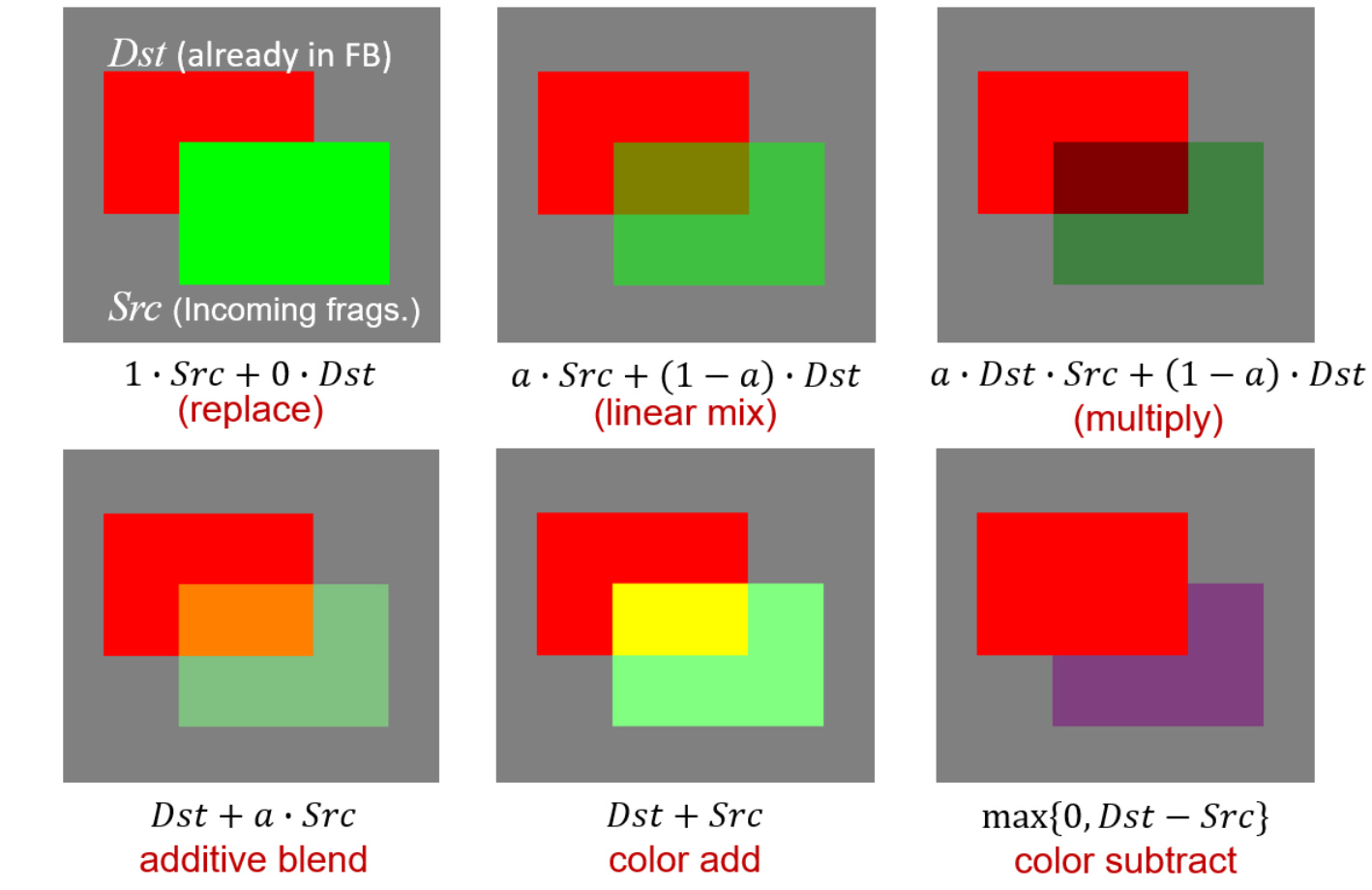
Transparent primitive rendering involves two elements: a) the definition of an alpha value for the pixel sample within the fragment shader and b) the specification of a blending equation to be used uniformly for the current rendering pass. The latter specifies how the alpha value is used in conjunction with the already accumulated color and alpha values. Graphics APIs provide specific calls to set up the blending equation, including how the alpha values are weighted and what operation to perform between the source (the current) fragment and the destination (the existing) pixel values. Some examples of blending operations are shown in the next figure:
The presence of a colored fragment in the final frame buffer is not only affected by its alpha value, however. The pixel coverage computed during primitive sampling is also used, linearly modulating the final mixing of the result with the frame buffer, regardless of the blending function used, since it represents "what portion" of the existing pixel is changed, without caring "how" the changed portion is affected.
It is important to understand that for most blending operations the order of primitive appearance in the drawing call queue is important; since the mixing of the source and destination values happens right after a fragment color and alpha value have been computed by the fragment shader, a "source" fragment becomes the "destination" value if the order the two primitives are rasterized is reversed. Certain operations are of course unaffected, such as pure additive blending, but in most other cases, different, order-dependent results occur. This is demonstrated in the following figure. The most significant implication of this is that the same object, without any alteration in its topology or primitive ordering will appear different under different viewing angles, since the order the fragments are resolved is not determined with respect to the viewing direction, e.g. back to front with respect to the eye space Z axis.

Furthermore, transparent rendering clashes with the simple hidden surface elimination method of the Z-buffer algorithm, as demonstrated below. In this simple example, two polygons are drawn with the depth test enabled in the GPU pipeline. In the left example, the transparent green polygon is drawn first. The depth buffer is cleared to the farthest value, so every pixel sample of the green polygon passes the test and is shaded. According to its alpha value, every fragment is blended with the gray background, as expected. But then arrives the red polygon, whose depth is farther from the green one’s. When attempting to rasterize the polygon, all pixel fragments that overlap on the image plane with the green polygon fail to pass the depth test and are rejected before having any chance to be (even erroneously) blended with the existing colors. On the other hand, if the red polygon came first, the depth resolution order would not cull the fragments of the part of the red polygon that is obscured by the green one, allowing this area to be blended and visible behind the green semi-transparent element.
Both problems are serious, especially when multiple transparent layers need to be drawn. One option to avoid entirely rejecting geometry behind transparent layers is to crudely sort the geometry into two bins and perform a separate pass for opaque and transparent geometry. Opaque elements are drawn first, proceeding as usual, with the depth testing and depth buffer updates enabled. This makes sense as the opaque geometry definitely hides all other geometry behind it, transparent or not. Therefore, if the closest opaque surface samples registered in the depth buffer are in front of any upcoming transparent fragments, the latter must be culled. Then in a second pass, all transparent geometry is rendered, but with a twist: depth testing is enabled, to discard transparent fragments behind the already drawn opaque geometry, but depth updates are disabled, so that no transparent fragment can prevent another transparent sample to fail the depth test because of it, regardless of the order of display. Needless to say, the order of appearance of the transparent fragments still affects the final blending result and transparency resolution is still order- and view-dependent. However, now we have contained the problem to transparent elements only.
Order-independent Transparency
To correctly draw transparent layers of geometry, surface samples must be first sorted according to image/eye/clip-space depth and then blended together from back to front, using the blending function activated, the each fragment’s alpha value and the respective coverage. This is exactly what the A-buffer (anti-aliased, area-averaged, accumulation buffer) algorithm does (Carpenter 1984), which has been around for many decades, even before the dawn of the rasterization architecture as we now it. Instead of storing a single (nearest) depth value, it maintains a list of all fragments intersecting a pixel. In modern instantiations of the method, each record of the sorted list contains the computed fragment color, depth, alpha and pixel coverage values. After drawing all elements, the list attached to each pixel is sorted (can be also sorted during fragment insertion) and the pixel color is resolved. In the original algorithm, whose primary concern was memory compactness and early termination, dealing mostly with opaque, antialiased geometry, the pixel resolve stage traversed the list front to back, maintaining a mask of "active" subpixel samples to resolve. When all sub-pixel samples were fully-covered, traversal was interrupted. Since nowadays an A-buffer implementation is primarily used for correctly handling transparency, the list is traversed back to front, blending the current fragment with the result of the blended, underlying ones.
The A-buffer technique is a lot more expensive than the simple Z-buffer method, as it involves, dynamic lists, more data per fragment and requires some sorting mechanism. A GPU implementation of the original method, using per-pixel-linked lists is possible, if one can guess how much memory needs to be (pre-) allocated, before running the algorithm. Unlike CPU memory, on-the-fly dynamic video memory allocation is not allowed and a quick fragment counting rendering pre-pass is typically used to record the amount of memory needed for the A-buffer. If this is to be avoided for performance reasons, either a very conservative budget is used (which is never ideal), or a clamped list is considered per pixel, storing up to fragment records, instead of an arbitrarily large number of them. Alternative multi-fragment rendering approaches also exist, that do not necessarily maintain an actual list and/or perform sorting on the fly (e.g. depth peeling). A comprehensive discussion about order-independent transparency (OIT) and the various multi-fragment rendering techniques to address it can be found at (Vasilakis, Vardis, and Papaioannou 2020):
Deficiencies of Rasterization
Rasterization is a very straightforward, fast approach to rendering and the basic pipeline operates in a divide and conquer strategy, rendering geometry in batches (draw calls), each primitive of a patch being processed independently, then each sample of a primitive being shaded independently. This enforced isolation makes the rasterization architecture extremely efficient and highly parallel, eliminating the need for global access to (and maintenance of) geometric data, as well as complex synchronization and scheduling on the hardware implementation. However, this narrowing of data visibility as information travels down the pipeline is also responsible for the many limitations of the basic rasterization method. Requiring vertex, primitive and pixel sample independence at each pipeline stage, means that these stages must be agnostic of other scene data; a vertex cannot access other vertices, a fragment shader cannot access other pixel samples but its own, a polygon is processed not knowing the full geometry of an object. This local-only access, prevents most algorithms that depend on global scene information to be applied within a shader. For example, when coloring triangle fragment, we can pass the light position and other attributes as uniform variables, but we have no way of determining whether the light sampled from the fragment’s position is intercepted by other geometry, causing a shadow to form. Things can become significantly worse if general global illumination is desired, where outgoing light depends on the incoming light from other surfaces, as is the case of reflected and refracted light.
To overcome such visual limitations of rasterization, in computer graphics we either abandon the rasterization architecture for the more general rendering approach of ray tracing (see further below in this unit), or resort to generating and maintaining auxiliary data via one or more preparatory rendering passes, which typically encompass the approximate and partial representation of the scene’s geometry, in order to make this information available during visible fragment shading. A prominent example of this is the shadow maps algorithm, detailed below, which enables the approximate yet fast light source visibility determination within a fragment shader. Another solution to the problem of indirect lighting is the use of pre-calculated information in the form of textures, such as environment maps and lightmaps (see next).
Simple "direct" rasterization of surfaces can also be inefficient when the depth complexity increases (many surfaces overlap in image space), since many shading computations may be waster to render fragments that are later overridden by samples closer to the viewpoint. Another issue stems from the lighting computations. Multiple light sources require either iterating over them inside the fragment shader, which introduces a hard, small limit on their number, or re-rendering the full scene once per light source, which is very costly. Furthermore, the rasterization of very small primitives, i.e. pixel- or sub-pixel-sized ones, incurs a penalty during the sampling process. The rasterizer, in order to compute necessary values to draw textured primitives (at least, the texture coordinate image space derivatives), rasterizes primitives in small pixel blocks and computes interpolated values for the samples even if these are not forwarded for display and shading. For small primitive footprints on the image, out-of-boundary samples will be evaluated often, which will be also subsequently re-evaluated for the neighboring primitives. Furthermore, the GPU hardware is optimized for processing few triangles with many pixel samples at a time, not the other way around. This has led graphics engine developers to seek ways to bypass the standard, fixed sampling system of the GPU for small geometry, implementing a software-based rasterization stack as a general-purpose compute shader that runs alongside conventional hardware rasterization8.
Rasterization-based Techniques
In this section, we present some important ideas and approaches to augment the capabilities of the basic direct rasterization architecture. A key element in most cases is the fact that the rendering of a complete frame needs not be done in a single drawing pass. Multiple passes can be used to prepare intermediate results and auxiliary image buffers that contain illumination and geometry information that can be exploited by a "final" pass to draw a picture with higher fidelity, support for more phenomena or increased drawing performance. The simplest such example is the two-pass approach to separately draw opaque and transparent geometry, as discussed above. In most cases, this process is not relevant to image compositing, as the intermediate buffers often convey information that is different in nature or coordinate system than the main pixel coloring pass. For example, one pass may prepare a sampled version of the scene as observed from the point of view of a light source (see shadow maps algorithm), or produce buffers of geometric attributes (see deferred rendering). Needless to say, most modern graphics engines implement multi-pass rendering with many different stages, combining results in a non-linear stage graph, often re-using partial results of previous frames as well or amortizing their creation across several frames.
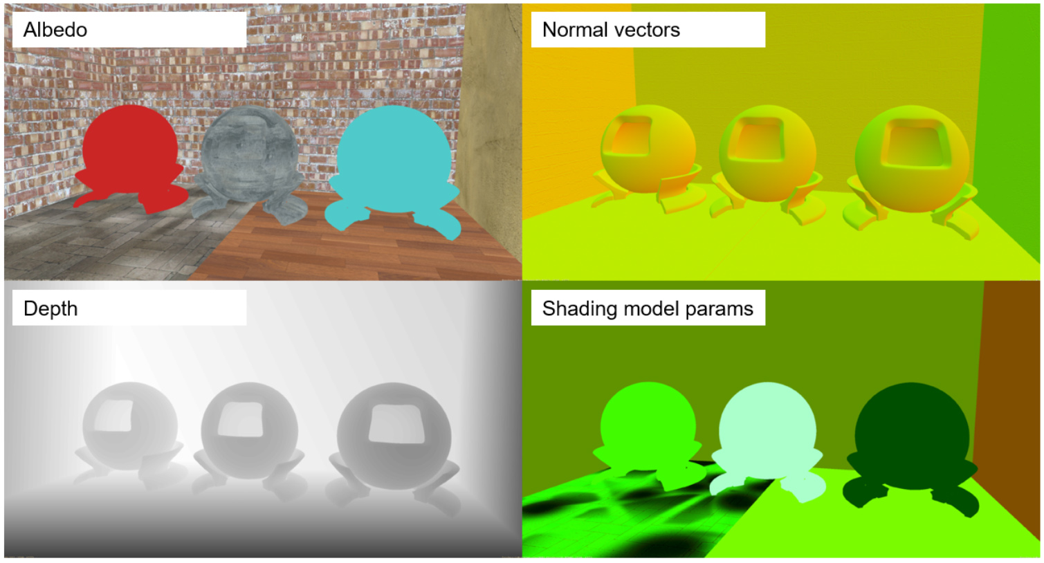
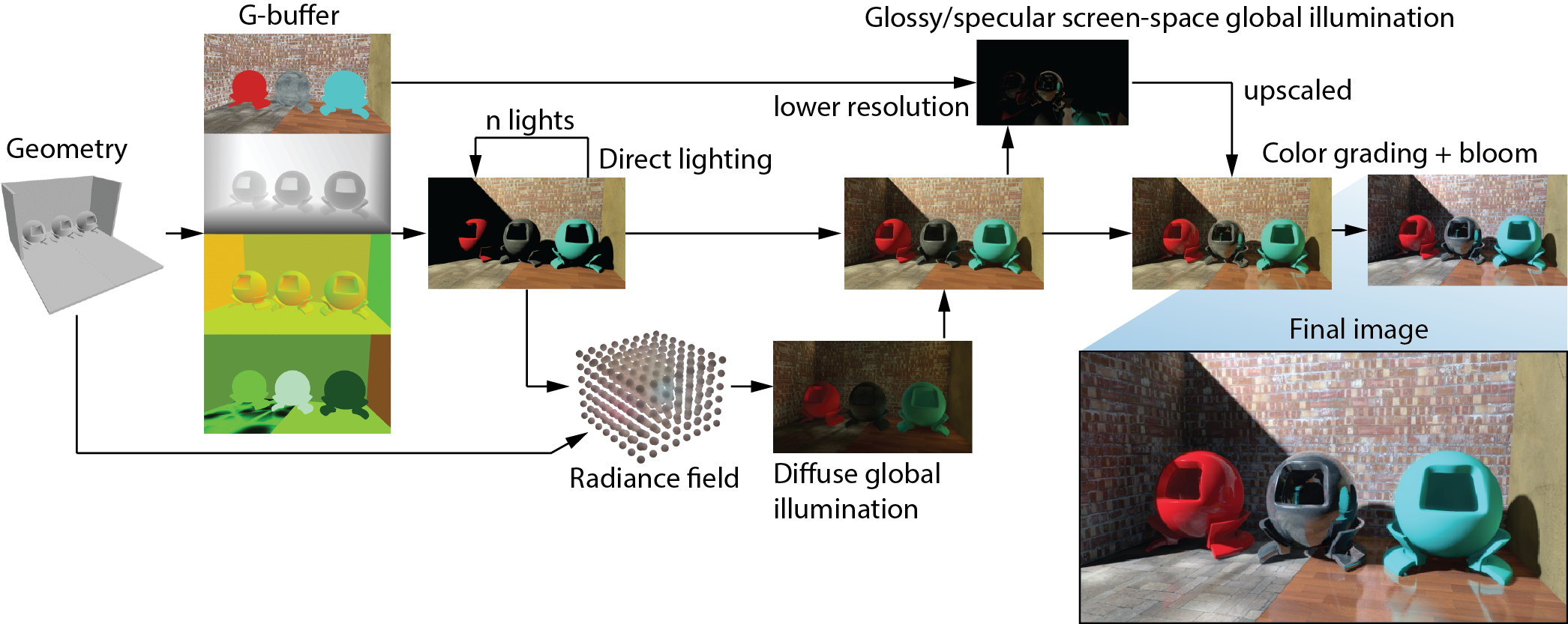
Deferred Shading
Deferred shading is a rasterization-based software architecture that was invented to address the problem of wasted and unpredictable shading computation load due to pixels being overwritten during hidden surface elimination. It delays (defers) shading computations until all depth comparisons have been concluded, performing shading only on truly visible fragments. To do this, deferred shading is divided in two discrete stages: the geometry pass and the shading pass. In the geometry pass, a number of image buffers are bound and recorded, collectively comprising the geometry buffer or G-buffer, all in one pass, with each channel containing a particular piece of geometric or material information. Apart from the default depth buffer enabled and prepared as usual, this information may include basic shading information, such as the RGB albedo, normal vector, metallicity, roughness and reflectance at normal incidence. The position and orientation of each fragment can be easily recovered in any global coordinate space (clip space, eye coordinates, world coordinate system) using a transformation matrix and the registered pixel location and depth, to perform shading computations in the next step. Additionally, other data may be also written in the G-buffer, such as interpolated velocity vectors, eye-space depth, emission, etc.
The shading pass is performed in image space, completely dispensing with the scene representation. The G-buffer attributes include all necessary information to run a local shading computation per pixel. To implement the shading pass, a quadrilateral covering the entire viewport is rasterized, and its fragment shading invocations are used to evaluate the shaded pixel, fetching the corresponding data from the G-buffer. Illumination from multiple sources can be implemented again inside a loop running in the lighting sub-pass, but also using separate draw calls per light. Now the second option is rather fast, as essentially two triangles are drawn per call. Furthermore, the area of effect of light sources has an often limited footprint on screen, facilitating the use of a different proxy geometry to trigger the lighting computations, further reducing the shading cost, as pixels guaranteed to be unaffected by the current light source are never touched.

The main benefits of deferred shading are the following:
Known and fixed shading cost, regardless of scene complexity. Shading budget is only dependent on image resolution, since only visible fragments get shaded.
Random global access to image-space geometric and material attributes of other visible fragments. This enables the implementation of many important screen-space algorithms to do non-local shading and filtering.
Ability to decouple the computation rate for different rendering passes over the G-buffer (decoupled shading). For example, lighting can be computed at 1/4 the resolution of the G-buffer, while screen-space ray tracing or bloom effects can be computed at an even lower resolution and then up-scaled.
However, there are certain limitations that come with the decoupling of the geometry rasterization and the shading. First of all, since only the closest (according to the depth test) fragments survive the geometry pass and record their values in the G-buffer, it is impossible to support transparency in deferred shading. For this reason, in practical rendering engines, deferred shading is performed for opaque geometry, which typically comprises most of the virtual environment, and transparent geometry is rendered on top of the prepared, lit result using as a separate direct (immediate) rendering pass. Transparent geometry is culled according to the prepared depth buffer of the opaque geometry, as usual.
The second limitation involves antialiasing. Certain techniques, an especially MSAA, are rendered useless with deferred shading, as they can only be applied to the geometry stage. Lighting is not antialiased. This is one of the reasons why MSAA has lost ground in practical game engine implementations, in favor of alternative, image-space techniques, which not only are compatible with the deferred shading pipeline, but also take advantage of the additional geometric and material information available through the G-buffer, to improve the filtering quality.
Tiled and Clustered Shading
Tiled rendering is a technique orthogonal to deferred shading. Its primary purpose is to limit the resources required to be accessed at any given time during rendering and is manly used to bound the number of light sources that affect a particular part of the image, in scenes with too many lights to iterate over efficiently. Tiled rendering, as the name suggests, splits the image domain into tiles and renders each one of them independently, after determining which subset of the shading resources truly affect each tile. A simple example is given in the following image. In this particular example, let us assume that the scene contains too many lights to be efficiently iterated over within a single pixel shader. So the pixel shader can only handle at most 4 light sources. We also make the assumption that most of the light sources are local and with low intensity, meaning that they have a limited range within which they practically contribute to any visible change in the scene’s illumination level. If we rendered the entire viewport at once, all light sources should have been accounted for. Failing to do so, by limiting the rendering pass to 4 sources, would mean that either we would need to cull a very high number of potentially important light sources, or repeat the lighting pass, until all quads of lights have been processed. When using tiled rendering, the projected extents (disk) of each source can be tested against the tiles’ bounding box. An array of up to 4 light sources can be created then for each tile separately, allowing the contribution of a higher number of light sources to the image, spatially distributed among different image tiles, at (nearly) the same total image buffer generation cost as a single 4-light rendering pass.
https://media.gdcvault.com/gdc2015/presentations/Thomas_Gareth_Advancements_in_Tile-Based.pdf.
Clustered shading is a generalization of the above stratification approach, were instead of considering a subdivision of the 2D image plane, tiling is applied to the three-dimensional space, usually the clip space. In this sense, a finer control of importance is possible and fewer resources are enabled per tile. Importance can be now tied to the distance to the camera position, meaning that for far away tiles along the Z tiling direction, different limits can apply. For example, for volumetric tiles closer to the viewpoint, one can accept more per-tile light sources to be rendered, reducing them or completely disabling them for distant tiles.
Tiled Rendering
Tiled shading is not not be confused with tiled rendering. Tiled rendering is a more drastic modification of the rasterization pipeline to directly operate on one image tile of the full frame buffer at a time, right from the start. The idea is to reduce the (hardware) resources required to produce a complete high-resolution frame buffer, by working on one smaller region at a time, requiring a fraction of the memory for all tasks (working output pixel buffer, attribute and fragment queues). Tiled rendering treats each tile as a mini frame buffer for the purposes of clipping. Primitives are split at the boundaries and their parts forwarded to the corresponding tile queues for rasterization, to avoid re-sampling polygons overlapping multiple tiles.
A beneficial side-effect of concentrating the effort of the software or hardware implementation of such a tiled architecture to a spatially coherent region is that data caching efficiency is drastically improved and flat in-tile shared memory access is now practical. As a consequence, tiled rendering is widely used in mobile and console GPU implementations, but also in desktop GPUs.
Decoupled Shading
Deferred shading is one form of decoupled shading in the sense that it separates the shading computational load from the complexity of the drawn geometry. Other forms include statically or adaptively decoupling the image resolution from the actual shading rate and texture-space shading. In the first form, shading occurs at a lower resolution internal frame-buffer and the prepared result is then upscaled to match the desired output resolution. Here, one of two things can be happen: a) Perform only specific expensive pixel shading calculations (e.g. glossy reflections) in low resolution and then upscale only these effects to the native resolution, maintaining a different rate for each shading calculation. b) Render the entire image at a lower resolution and predict an upscaled version of it. The latter, which is based on theory and methods related to super-resolution video, relies on designed or learned predictors, typically using neural networks (see for example NVIDIA’s DLSS), to exploit previous frames and G-buffer information alongside the low-resolution frame buffer, to derive a well-informed high-resolution version of the current frame.
Texture-space shading is an orthogonal approach to the above, where instead of shading the sampled pixels of the image plane, shading samples are taken and computed on a texture image covering the geometry. The shaded textures are then used along with the conventional ones to draw the final image buffer, but with a far simpler (and faster) pixel shader, which only uses the computed lighting already stored in the texture-space rendering pass. In this method, the image buffer(s) correspond to the unwrapped textures that cover the objects (texture space) and their resolution can be significantly different than the output frame buffer. The shading density is also not constant with respect to the output frame buffer sampling rate, but can vary according to geometry feature importance, object distance, etc., providing many degrees of freedom to control shading quality versus speed. Texture-space shading also offers many opportunities for temporal re-use, as view-independent lighting information can be re-used across multiple frames. Despite its many welcome properties, texture shading also has generally higher memory requirements, as it needs to maintain separate shading textures per object instance (shading is not shared among instances of the same object) and also requires the preparation of a bijective texture map, which is not trivial and may introduce its own artifacts. However, in a more limited form, texture-space shading is very common in real-time rendering, to "bake" (pre-compute) or update on the fly, possibly amortized over frames, heavy illumination computations, such as diffuse global illumination (see light maps below).
Decoupled shading can also refer to shading in any other parametric space and not necessarily a planar one. For instance, shading can be performed in object space, using volumetric representations, possibly in a hierarchical organization to allow for high spatial resolution, when needed. Furthermore, even simple forms of image-domain decoupled shading can adopt a non-uniform sampling rate, as is the case of foveated rendering, where sample density is higher near the gaze direction of the user and becomes lower in regions where the peripheral vision is more prominent.
https://www.geoweeknews.com/blogs/apple-bringing-3d-sensing-ar-vr-iphone.
Visibility and Shadows
Visibility between two points in space requires the existence of knowledge about the location of all other geometry that may cross the straight line connecting them, since we need to check for the intersection of that linear segment and the representation of the potential occluders. However, the rasterization pipeline operates locally on single primitive samples in isolation. Therefore, this global geometric information must come from outside the rendering pass that the visibility query is invoked from. Remember, it is very seldom that a visualization task involves only a single rendering pass. We more often than not perform one or more preparatory passes to produce temporary auxiliary buffers to be used later in the frame generation pipeline. This is exactly the idea behind one of the most popular single real-time methods used in almost every interactive rendering application: the shadow maps algorithm. Below we present the core idea and some extensions and variations, but also attempt to cover other visibility ideas associated with rasterization.
Shadow Maps
The shadow maps algorithm, which by design works for punctual lights with conical emission (a "spotlight") is based on a very simple idea: if something is lit, it is accessible by the light source and therefore it should be "visible" from the light source’s point of view. Since the lit primitive parts are visible to the light source, they must therefore be the closest to the light source. So if one were to render an image using as "eye" the location of the light source and as viewing direction the spotlight’s emission cone axis, the closest samples registered would be all samples on lit surfaces. We call this light source’s depth buffer, a shadow map (see next figure).
The algorithm operates in two discrete stages. Given a single light source, in the first stage, the rasterization pipeline is set up so as to render the scene from the light’s point of view, as detailed above. Since we are interested in forming just the shadow map, i.e. normalized depth of geometry from the light position, any color information typically produced by a pixel shader is irrelevant in the most basic form of the method, and is therefore completely ignored. No color buffer is enabled and no color computation is performed. In stage two, we switch to the camera’s point of you to render the shaded image as usually. Here we query the shadow map to determine whether a shaded point is in shadow or not. We do so by transforming its position to the same coordinate system as the stored shadow map information and then checking whether the new, transformed sample’s is farther from the recorded depth in the shadow map for the same and coordinate. If this is the case, the sample cannot be lit (in shadow), since some other surface is closer to the source and intercepts the light. Otherwise, the light source is visible (no shadow). The transformations required to express a camera-view image sample to the light source’s normalized space are all known: We have explicitly specified the world to camera and the world to light transformations (both systems are known) and we have set up the projections for both cases. The transformations are also by design invertible. The concatenated transformation matrices are supplied as uniform variables to the fragment shader and th process is quite fast.

The shadow maps algorithm is a prominent example of a technique where actual geometry is approximated by partial and sampled version of it. It is clearly also a case of decoupled "shading": we run a fragment shader to compute the shadow map which has a different and uneven sampling rate with respect to the camera-space pixel generation rate. In fact, the latter is actually a source of error in the process and one of the negative aspects of the method.
There are several positive aspects of using shadow maps for light source visibility testing and in fact, for several low- and mid-range hardware platfroms, shadow maps constitute the only viable real-time solution, despite the advent of ray tracing support at the hardware level of modern GPUs. Some of the advantages are as follows:
Full hardware support, even in low-end devices, since it only requires simple rasterization of primitives to work. Directly supports HiZ mechanism, where available.
Decoupled and scalable rendering quality. Shadow maps resolution is independent from the the main view resolution and can be tuned for trading performance and quality.
No extra geometric data are produced and maintained in the GPU memory (e.g. acceleration data structures in the case of ray tracing). The shadow map fills the role of the scene’s geometric proxy for the task of visibility testing.
Directly compatible with the primary view in terms of representation capabilities. They both use rasterization and fragment-based alpha culling, supporting the same primitives and effects.
Simple and intuitive 2-pass algorithm with linear dependence on scene complexity.
Shadow maps are easy to combine with and integrate in other effects, such as volumetric lighting (e.g. haze, godrays).
On the other hand, there are several limitations and problems that come with a) the specific setup for the light projection and b) the fact that shadow maps are a discretized representation of the virtual world, causing sampling-related artifacts and precision errors. More specifically:
Simple shadow maps require projector-like light sources. A single-pass shadow map generation stage with the most basic setup, can only capture shadows from projector-like (spotlight) or directional light sources, since it requires the configuration of a regular projection (perspective or orthographic, respectively) to record the closest to the light source geometry samples. Omni-directional light sources must render the depth information in more than one shadow map buffers, such as cubemap shadow maps and dual paraboloid shadow maps. Using additional projections fortunately does not imply the emission of the geometry multiple times in modern hardware, since replicating the geometry and "wiring" it via different projections to multiple frame buffers can be done with geometry instancing and/or layered rendering in a geometry shader. Still, even this, breaks the simplicity of the algorithm and incurs some additional cost.
Only work for punctual or directional light sources. Shadow maps with a perspective projection require a single center of projection. It is therefore impossible to query visibility of samples distributed over an area light source. The only options for approximating area lights are: a) temporally change the center of projection and respective transformation and average (blend) the results in camera image space. This incremental approach can work for stable views only. b) Fake the area light by jittering the camera-space fragment position within the fragment shader and combine visibility samples and c) jitter the shadow-map (image) space samples and average the visibility results to mikic soft shadows. The latter is also used for shadow mapping antialiasing (see below).
Cause under-sampling and pixelization artifacts. Camera fragments are produced with a specific screen-space sampling rate and are then unprojected, affinely transformed and re-projected to the shadow map space. This means that the resulting sampling positions are generally completely incompatible with the rasterization rate with which the shadow map has been produced. Severe aliasing can be produced due to the density of the projected camera fragments being either higher than the shadow map pixels, resulting in pixelization artifacts, or lower, causing under-sampling errors and flickering. The problem is demonstrated in the following figure (areas highlighted with green). Both problems are partially alleviated by sampling the shadow map using percentage closer filtering (PCF) or some similar visibility estimator. PCF draws multiple depth samples, instead of one, in the vicinity of the projected fragment onto the shadow map and averages the visibility decisions for each shadow map depth. Simple texture filtering on the shadow map, which is a depth image, does not work.
Cause visibility inconsistencies and artifacts. Due to the different sampling rate of the camera and light space image domains, camera samples falling in-between shadow map pixel centers do comparisons with interpolated values, which, due to projection, linear interpolation and numerical imprecision, can be offset either back or front with respect to the true surface boundary. This means that fragments on the lit side of surfaces may actually fail the visibility comparison by a small value, causing what we call the "shadow acne" effect, i.e. crawling random or systematic spots of shadowed fragments on lit surfaces. This problem is demonstrated in the following figure in the regions highlighted with red borders. An obvious corrective measure to this is to add a small error margin in the depth comparison between the projected fragment depth and the recorded shadow map depth, called the "shadow bias". However, doing so uniformly, can cause the bias to affect all depth comparisons, making the shadows detach themselves from the occluding geometry, an effect known as "Peter Panning", as it brings to mind the ability of Peter Pan’s shadow to detach itself and roam independently. The error is more evident at places where the shadows are more oblique. See the next figure for a demonstration of the problem (areas highlighted with red). Certain improvements to the constant shadow bias approach have been proposed, such as adapting the bias amount according to the relative relative slope of the surface with respect to the light incident direction, but with limited success, resulting in some form of manual adjustment to be typically required. Recently, the solution that most game engines employ is to aggressively set up the bias to get rid of the shadow acne and compensate the shadow shift by filling in the missing occlusion with some other technique (see contact shadows below).

Screen-space Ambient Occlusion
Despite the fact that ambient occlusion (AO) (see Appearance unit) is not a physically correct illumination technique, it has long been used and improved as a helpful shadowing effect to accentuate the appearance of unlit geometric features by dimming approximate indirect light at statistically low-visibility areas. Computing ambient occlusion generally involves shooting rays at the hemisphere above a point and checking for intersections with other parts, usually within a limited distance range . However such a way to compute AO is not directly compatible with the rasterization pipeline, requiring the pre-computation and storage of AO in textures (AO is scalar, so it occupies a single image channel) and prohibiting its application on dynamic virtual environments. With the advent of more powerful GPUs, per-object static AO could be pre-computed and dynamically blended in composited scenes or, more practically, discretized distance fields surrounding the scene elements were pre-computed and queried in real-time to approximate the desired effect. However, such volume-based approaches are still quite demanding, especially if updates to the distance fields are required. For games, where corners need to be cut in terms of visual fidelity and accuracy to sustain a high frame rate, a far simpler and cost-effective technique was devised: screen-space ambient occlusion (SSAO).
SSAO is based on a very simple idea. Since the depth buffer of a rasterized frame constitutes a sampled approximation of the visible geometry, one could sample a surface-aligned hemisphere of radius and centered at the fragment position to count how many of the sample positions lie "behind" the depth buffer. That percentage could be directly interpreted as AO and used to shade the current fragment. SSAO requires the use of a deferred shading pipeline, since in order to compute the AO for a fragment, access to correct nearby depth values must be feasible during shading. In the early implementations of SSAO a full sphere was sampled, scaling and clamping the result, because it was faster to do so. Based on this simple statistical method, many more accurate methods have been subsequently devised, which are used even today to enhance the appearance attained by modern real-time rendering solutions.
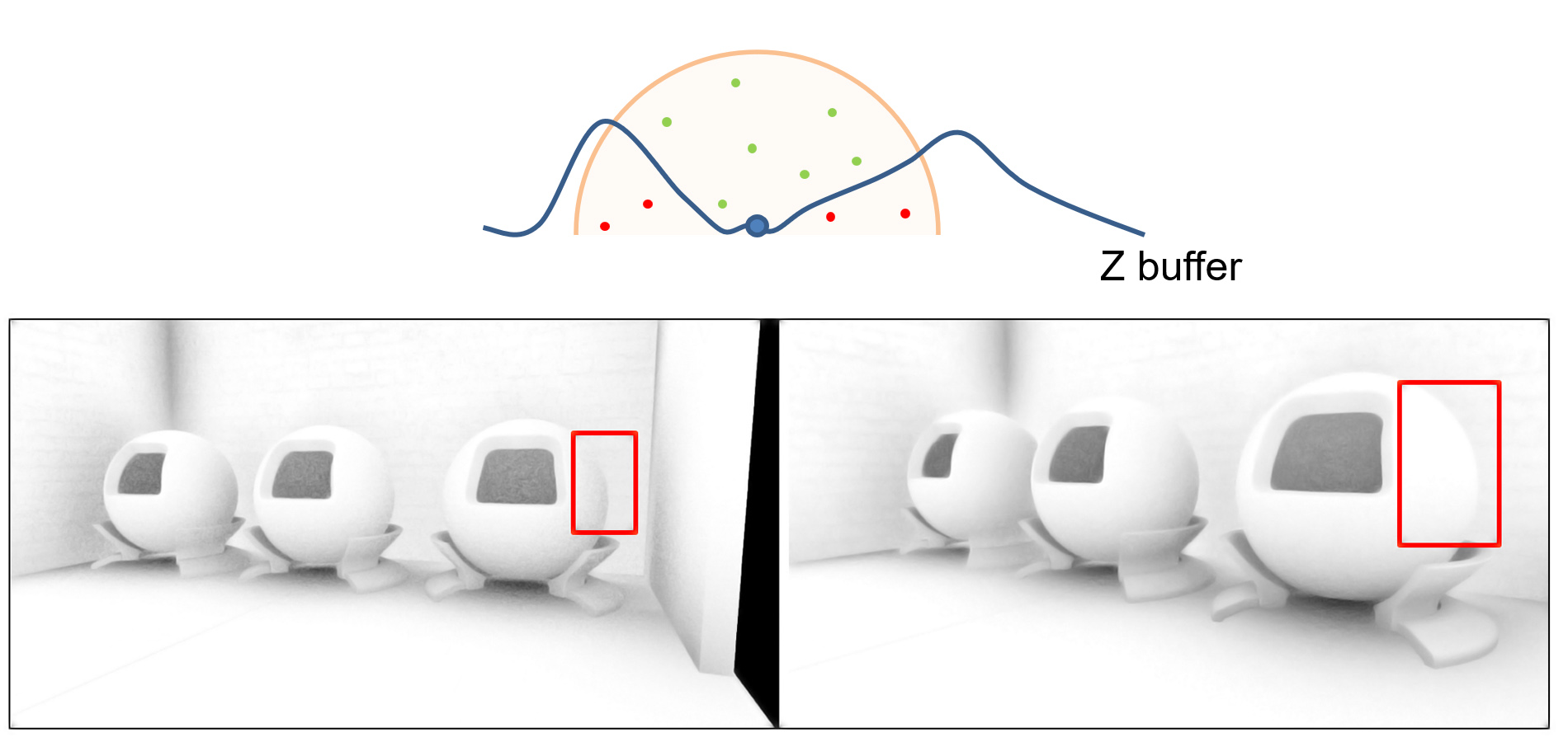
SSAO generally suffers from view-dependent artifacts. Since the sampling of the depth buffer relies on the in-view surviving fragments, changing depth at object discontinuities, the disregard of out of view geometry and over-estimation of AO behind thin structures makes the computed AO change as the camera moves or objects appear in or disappear from the view. Stabilization solutions exist, including rendering a wider image buffer than what is visible for the calculation of AO, clamping the AO sampling region with the image space (Bavoil, Sainz, and Dimitrov 2008) and the computation of AO based on fusion of sample queries from multiple views (Vardis, Papaioannou, and Gaitatzes 2013). Additionally, using multi-layer depth information can drastically improve the computed AO quality, but at an expense of time and resources, which are not easily justifiable by the impact of AO in typical applications.
Contact Shadows
Contact shadows refers to an occlusion detection technique that operates on the near-field meso-scale geometry of a shaded point. It attempts to recover visibility information that is hard to attain with other approaches, such as shadow maps. It is usually applied as a complementary method to the shadow maps algorithm to fill in shadows near the visible surfaces, where depth comparison is problematic and uncertain. Remember that in order to correct shadow acne, a small bias was introduced, inevitably shifting the shadowed region a small distance away from the occluding geometry. Contact shadow operate to close this gap and recover missed shadows.
Contact shadows estimation typically operates in screen space, not unlike SSAO. However, contrary to SSAO algorithms, which sample the entire hemisphere above a shaded point, contact shadows draw a small number of successive samples along the direction that connects the shaded point and the light source position, within a limited distance. Each sample’s screen-space depth is checked against the depth buffer’s corresponding value and if at some point it becomes larger (farther) than the depth buffer distance, this means that the line of sight towards the light source is interrupted by geometry registered in the depth buffer, signaling a termination of the ray marching iteration and the report of a positive occlusion. The process is illustrated in the following figure.
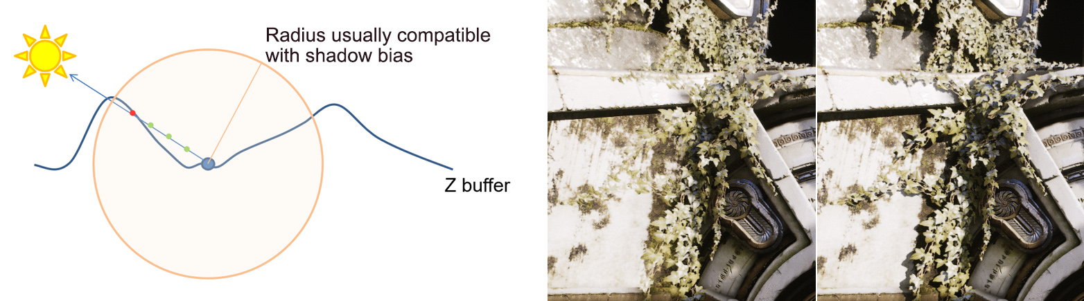
Ray Tracing
Casting Rays
Ray tracing is a general and versatile algorithm that samples the virtual environment by constructing rays, starting from a point in 3D space (the origin) and pointing towards a specific direction, and then casting the ray into the environment to perform an intersection test between the ray and the primitives constituting the virtual world. Upon discovering the closest hit to the origin, the search is terminated and the attributes of the hit point are used to perform any shading. The computed illumination at the hit point can then be carried back to the point of origin to contribute to an image synthesis task or any other simulation.
But let us first examine a simple replacement image synthesizer for the rasterization pipeline. We need to construct at least one ray per frame buffer pixel, starting from the center of projection and passing through a point on the image plane within the area of effect of each frame buffer pixel. For a single ray per pixel, typically the center of each pixel on the raster grid is chosen. The rays are generally defined in world space coordinates, since ECS or clip space coordinates make no sense and provide no benefit as a common reference frame in ray tracing. With no other provision in place, each ray is then tested for intersection with all primitives of all objects and for each valid intersection with a primitive, the hit location is examined to check whether this is the closest one to the origin discovered so far, or not. If the current hit point is the closest one so far, its attributes replace any other hit point data maintained so far for this ray. When no other intersections exist for a particular ray, the closest hit data (if any) are used for computing the local shading and the resulting color is registered on the frame buffer pixel that corresponds to the ray.
This simple image synthesizer was proposed quite some time ago (Appel 1968) and is equivalent to a rasterization-based immediate shading pass. The rasterization pipeline operates on geometric primitives and fills arbitrary and overlapping locations in the frame buffer with color information. In a general sense, it constitutes an object-to-screen space image synthesizer. Sorting (hidden surface elimination) is also performed in image space, using the Z-buffer algorithm. Ray casting, as described above, in fact operates in exactly the opposite manner, i.e., it is a screen-to-object space image synthesizer. Hidden-surface elimination (in object space and not image space) happens as an integral part of this process, because the ray traversal needs to discover surface interfaces closer to the ray origin, while it travels through the three-dimensional world, to report a meaningful hit.
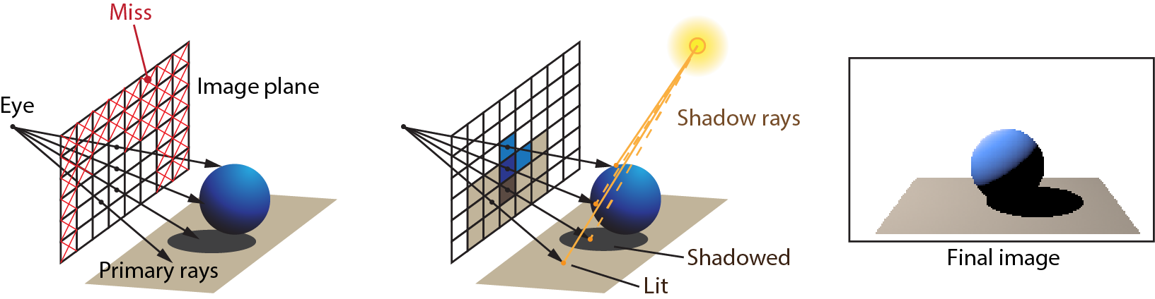
In this simple ray casting method for image synthesis, light visibility can be determined exploiting the same ray casting mechanism used for the primary rays, i.e. the rays cast from the camera center of projection; a ray is cast from the hit point on the nearest surface to the camera that is about to be shaded, towards the light source. If any surface is encountered between the origin and the distance to the light source, the ray queries are terminated and the origin is declared to be in shadow. This is very powerful: tracing rays in the virtual environment is just a very generic mechanism to explore and sample space, detecting collisions with the geometry (ray hits). Implementation-wise, once we have established a way to trace rays with arbitrary starting points (ray origins) and propagation directions, we can construct paths in 3D space formed out of segments connecting hit points, over which light can be carried within a simulation system. Obviously, the notion of following a path of light and calculating its behavior at the interface between materials has existed long before the beginning of the computer graphics era. Electromagnetic wave transmission theory, but most of all geometrical optics and the laws of reflection and refraction, provided the framework for the study of light—object interaction in the physics domain, a long time before the inception of ray tracing as a computer algorithm.
A Simple Recursive Algorithm
Although the ray-casting mechanism to display a three-dimensional scene with hidden surface removal as an alternative to scan-conversion is attributed to Appel (Appel 1968) and Goldstein and Nagel (Goldstein and Nagel 1971), an integrated approach to recursively tracing rays through a scene via reflection and refraction was proposed later by Whitted (Whitted 1980). It combined the previous algorithms that shot primary rays from eye point toward the scene until they hit a surface and then illuminated the intersection points with the recursive re-spawning of new rays from these points.
The principle of the algorithm is quite simple: For each pixel, a primary ray is created starting from the eye point and passing through the pixel. The ray is tested against the scene geometry to find the closest intersection with respect to the starting point. If the ray misses the geometry, a background color is evaluated and returned. When a successful hit has been detected, a local illumination model is applied to determine the color of the point according. To this end, shadow rays are cast towards the light sources in order to determine whether the hit point is lit or not. If any surface is intersected by the shadow ray (not necessarily the closest), the query is terminated and the point is in shadow. Next, a maximum of two new rays are spawned from the hot point: If the material of the surface hit is transparent, a secondary refracted ray is spawned. If the surface is reflective, a secondary ray is also spawned toward the mirror-reflection direction. Both secondary rays (reflected, refracted) are treated the same way as the primary ray; they are cast and intersected with the scene in a recursive manner. Thew process is illustrated in the following figure.
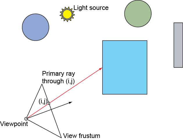
Each time a ray hits a surface, a local color is estimated. This color is the sum of the illumination from the local shading model as well as the contributions of the refracted and reflected rays that were spawned at this point. Therefore, each time a recursion step returns, it conveys the cumulative color estimated from this level and below. This color is added to the local color according to the reflection and refraction coefficients and propagated to the higher (outer) recursion step. The color returned after exiting all recursion steps is the final pixel color.
Rasterization-based rendering in its pure form disassociates the color and shading of a particular surface area from the existence of other objects in the same environment. Shadows, reflected and refracted light on surfaces, need to be simulated or approximated separately and fused as color information in the final composition rendering pass. Ray tracing, on the other hand, integrates all calculations that involve the scattering of light in one single and elegant recursive algorithm.
The recursive ray-tracing algorithm can be summarized as follows. Here we define a C++ function named raytrace, which is invoked every time a new ray needs to be evaluated for intersection with the geometry of the scene (the world variable).
Color raytrace( Ray & r, int depth, const Scene & world, const vector <Light*> & lights )
{
	Color color_refl, color_refr, color_local;

	// Terminate the procedure if the maximum recursion depth has been reached.
	if ( depth > MAX_DEPTH )
	    return Color(0,0,0);

	// Intersect ray with scene and keep nearest intersection point
	int hits = findClosestIntersection(r, world);
	if ( hits == 0 )
		return getBackgroundColor(r);

	// Apply local illumination model, including shadows
	color_local = calculateDirectIllumination(r, lights, world);

	// Trace reflected and refracted rays according to material properties
	if (r.isect.surface.material.roughness == 0.0)
	{
		Ray refl = calculateReflection(r);
		color_refl = raytrace(refl, depth+1, world, lights);

		if (r.isect.surface.material.transparency > 0.0)
		{
			refr = calculateRefraction(r);
			color_refr = raytrace(refr, depth+1, world, lights);
		}
	}
	return color_local + color_refl + color_refr;
}
The depth of the recursion, i.e., how many times new rays are spawned, is controlled primarily by two factors: First, if the ray hits a surface with no transparency or mirror-like finish, no new rays are generated. Second, to prevent an uncontrollable spawning of rays in highly reflective or transparent environments, a maximum ray-tracing depth is usually defined. The following figure shows a comparison between renderings with a different maximum ray-tracing depth. Early ray pruning results in very wrong images for certain scenes. In this particular example, a polished sphere is placed inside a glass case. This particular ray tracing implementation performs a local illumination evaluation only on non mirror-like surfaces (which is typical). With few recursive steps, shadow rays from surface layers nested deep into the transparent geometry fail to reach the light source (here the sky dome), resulting in under-illuminated areas. From a maximum depth of 6 and above, the image begins to look plausible, despite the fact that subtle effects are still missing (e.g. see the secondary reflections of the metallic ball on the inside of the case in the transition from depth 6 to depth 7).
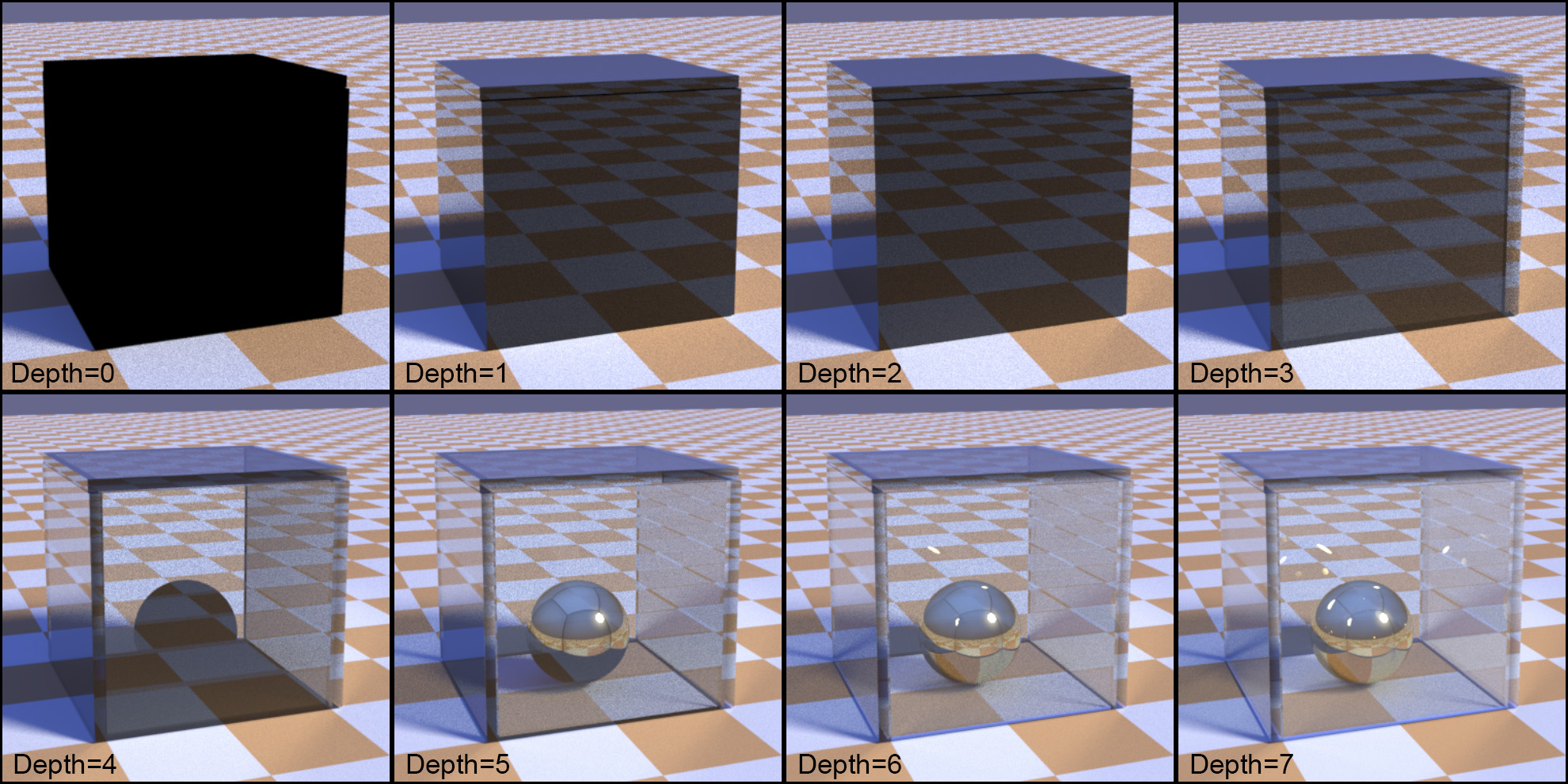
Examining the ray traced example above, several observations can be made:
The Whitted-style recursive ray tracing only addresses indirect lighting from specular events, i.e. from mirror-like surfaces, where light can only be reflected and transmitted in a single direction. Many early ray-tracing renderers used this kind of "too clean" path generation mode, resulting in unrealistic looking environments and requiring additional global illumination simulation methods to separately handle other types of scattering events (see for example the radiosity method).
All conventional ray queries, i.e. primary rays from the camera and secondary rays for indirect lighting, need to report the closest intersection. This means that in a naïve implementation, all objects and all their primitives must be examined to obtain an intersection point (if any) whose distance to the origin is the smallest one. We will see next that it is impractical to perform such an exhaustive search and special data structures are employed to accelerate the process in a "branch and bound" manner.
There is a special type of ray query used for visibility testing in the above algorithm, the shadow ray query. This type of search for intersection can terminate the moment it detects any hit and does not have to continue until the closest one is found. Here we only need to check whether a line segment connecting two points is interrupted by an obstacle. Therefore, such a ray query is generally faster to perform, as it terminates early.
A transparent piece of geometry, even if it is very clear, should still prevent a shadow ray from passing through and reaching a light source sample. This is because, unlike the way transparency works in rasterization as a blending factor, when encountering transparent objects in ray tracing, the surfaces represent an interface to a solid mass of an object and a transition from one index of refraction to another. This means that in general rays will change direction9, exiting from the other side from locations not on the extension of the incident ray. Therefore, it is wrong to assume that casting a shadow ray straight through a transparent medium would follow the true path of light coming the other way from the light source.
Terminating the recursion early, at any user-imposed depth introduces bias, i.e. the convergence of the rendered image to a result, whose illumination differs from the expected illumination in a physical sense. We have no way of determining, at which depth there is some guarantee that there is no significant energy contribution from going one step further. Keeping track of a ray’s importance (strength) as it diminishes by scattering on the environment may seem as reasonable stopping criterion to terminate ray tracing at a depth where this factor is too small. However, in many environments this is difficult to predict.
Ray Tracing Rendering Pipelines
In most application cases, it is both desirable and possible to decouple the application logic from the mechanism that actually traces rays in a virtual environment, leading to the design of a specific ray tracing architecture or back end. There are several reasons why this is important, starting from the fact that the ray tracing task itself can become quite elaborate in realistic scenarios (see accelerating ray queries below). Second, and perhaps most importantly, the ray tracing mechanism is abstract and generic enough to be clearly separated and reused in different contexts, even in non-visualization tasks. For example, we can employ ray tracing to do collision detection, acoustic simulation, nearest-neighbor queries and so much more. Third, nowadays, ray tracing queries are parallelized and tightly supported and accelerated by graphics hardware and specialized software libraries, distancing further the core ray tracing functionality from the final application logic. Such a ray tracing architecture, which frequently combines both hardware and software elements the same way rasterization does, has its own unique operation, with several stages being opaque or accessible for customization and modification.
As implied above, there are four ray tracing events that are important for the life cycle of a ray and the way it interacts with the geometry. First, there has to be a clear stage where a ray is first born and subsequently evolved into a (potentially branching) path to track light contribution. In the simple Whitted-style ray tracing algorithm, this corresponds to the casting of rays from the camera point of view. However rays can be initiated from other locations in space, depending on what lighting simulation needs to be implemented. For instance, one could attempt to trace photons from the light emitting surfaces or trace incoming light from multiple planar sensors.
The next two events that need to be handled are associated with the interaction of the rays with the 3D representation of the environment (not necessarily surfaces). Specifically, we need to react when a ray has been intersected with the scene and the closest hit is reported. This is a very important event, as a path segment is formed between the origin of the current ray and the next accessible location in the direction the ray is cast. For typical surface intersections, this signifies the next scattering event on the interface between to materials (e.g. air and glass), where we need to compute a new ray to trace. In order to locate the closest hit, a ray is potentially successfully intersected with multiple other valid hit points, which may or may not be the closest to the origin, as this is something to be determined after all intersections have been identified. We have seen in the ray casting and recursive ray tracing examples above that we typically cast rays from the shaded points, where the scattering events are tracked, towards the light sources to determine the light source’s visibility. If these shadow rays are interrupted at any point in the interval between the shaded point and the light sample position, visibility is zero. Therefore, there is a need to be able to respond to any hit ray intersection events as well, to terminate a ray intersection early or perform other filtering or counting operations.
Finally, we need to define the behavior of the ray tracer when a ray hits nothing, i.e. on a miss event. A typical example in rendering is the handling of rays when they are directed towards the background, after missing all geometry. There, we must clearly specify what is the radiance returned by the infinite surrounding void space, given a ray’s direction.
An example of such a ray tracing architecture is shown in the next figure. Bear in mind that contrary to the rasterization pipeline, which has been around for many decades and has been pretty much standardized to adhere to the OpenGL, DirectX and Vulkan specifications, the ray tracing architecture ecosystem is rather young, despite the fact that ray tracing has been around for nearly as long as rasterization as a viable image synthesis paradigm. Common to all implemented solutions is the abstraction of the specifics of ray query scheduling and invocation. All implementations support at least one form of ray query acceleration data structure (see next) and all generic application programming interfaces provide "hooks" to implement and call your own code to handle the above 4 types of ray events.
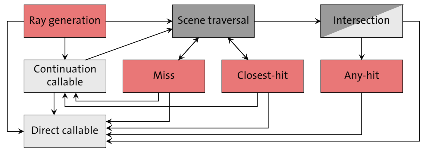
The closest hit event is typically the main point where a) shading takes place and b) new rays are potentially spawned to continue the exploration of space by forming a path of connected hit points. The "any hit" event is not always handled explicitly, unless specific code must be written to modify the results of the query. For example, rendering perforated geometry that uses a texture mask to mark specific parts of the primitive as invisible or "pass through", requires the invocation of an event handler at every hit, to check whether the particular location is a confirmed valid hit or must be rejected as a hit (and the ray should continue as if the hit never occurred), according to the opacity mask.
Accelerating Ray Queries
In a ray tracing-based image synthesizer, by far the most frequent computation is the intersection test between a primitive and a ray. Millions of rays are typically spawned to synthesize a single image and each one has to be tested against all scene primitives, which may amount to many millions themselves. The problem of exhaustively computing all these intersections can quickly become intractable. In general, there are three ways to improve performance in a ray tracing environment:
Cast fewer rays. This can be translated into selectively or adaptively spawning new rays, only where there is a high probability that the new rays will actually contribute to the improvement of the final result. Such a strategy is very common and, if properly exploited, can result in large savings in computation effort, without biasing the final output. Another way to interpret this is to replace typical infinitesimal rays with other geometric primitives, each representing an entire bunch of rays, replacing individual ray tests with a single (yet more complex) primitive-to-primitive test. Indicative representatives of such a strategy are beam and cone tracing (Amanatides 1984). Due to the need to address many corner cases, the complexity of intersections and the loss of generality in the potential combinations of primitive-to-primitive intersection testing, such approaches are not very popular in generic applications.
Make intersections faster. Modern ray tracers interact with specialized GPU hardware (ray tracing cores) to expedite common ray intersections, such as ray-triangle intersections, since triangles are the most common and generic primitive used in 3D modeling and geometry processing. In general, ray tracing engines support intersections with arbitrary geometry (or volumetric data) by allowing programmers to specify custom intersection functions for user-defined primitives. This can introduce a significant speed improvement when rendering well-defined parametric and analytical surfaces, where a single primitive (e.g. a sphere) can be directly and exactly queried for intersection instead of testing a ray against an approximate triangular mesh representation of the object, containing many triangles. Additionally, ray queries are inherently independent (one ray against the virtual environment) and therefore, trivially parallelizable. Modern GPU and CPU implementations trace rays in batches, scheduling the ray query execution to run in a highly parallel and synchronous manner.
Cull ray queries early. This is an important improvement and one with the most significant impact on performance. All ray tracing engines employ some form of "branch and bound" search mechanism for ray queries, which boosts performance by orders of magnitude, by safely discarding entire sections of the virtual environment, when attempting to compute an intersection with candidate primitives, based on the relative spatial relationship between the ray and the geometry. This is a field of active research which has leveraged both generic and specialized hierarchical data structures to index space and de-linearize the search for the closest intersection. Bounding volume hierarchies are the most popular choice for such a hierarchical indexing, since they tend to minimize the size of bounding volumes thus decrease the chance that a ray query with a bounding container will yield a false positive intersection test with it.
Bounding Volume Hierarchies in Ray Tracing
In the geometry representation unit, we have explained that complex geometry can be decomposed into smaller and smaller, spatially coherent clusters of primitives whose bounds can be organized hierarchically. In the context of ray tracing, these supporting bounding volume hierarchies can be effectively used to interrupt the search for collisions between a ray and a cluster of primitives (Meister et al. 2021); if the ray does not intersect the bounding volume of the cluster, the (wholly) contained primitives cannot be possibly intersected and are directly skipped. The same holds in the case of bounding volumes contained within other bounding volumes in the hierarchy, thus skipping large sections of space and most of the primitives therein. This is demonstrated in the following illustration. The various schemes that build hierarchical clusters of bounding volumes and linked primitive clusters and provide traversal for the ray queries are collectively called acceleration data structures (ADS).
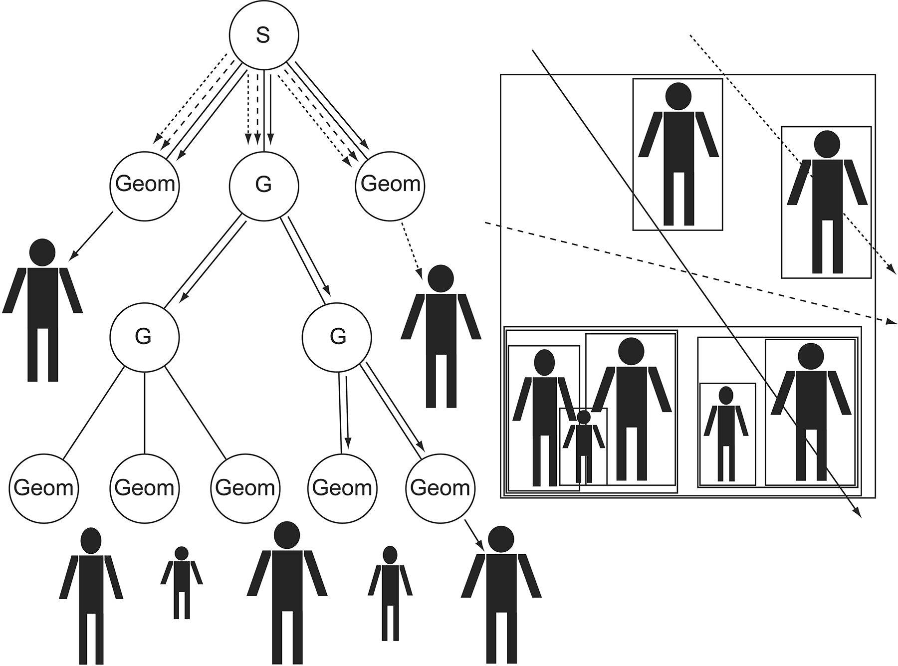
Building a high-quality ADS is crucial for the performance of the ray-scene intersections. The construction of an ADS attempts to either agglomeratively combine primitive clusters (bottom-up strategy) or split space (top-down strategy) using a strategy that attempts to optimize at least two of the following:
Traversal depth. Building a hierarchy that is too deep (high), i.e. having too many branching levels, results in a lot of computational effort navigating the ADS, before locating the actual primitive clusters. This introduces a significant average overhead and a source of divergent parallel execution on an SIMD (single-instruction, multiple-data) architecture, such as the shading multi-processors of a GPU. In many ADS implementations, binary subdivision schemes are used, but it not uncommon to also consider higher branching factors, in order to make hierarchies wider, but shorter.
Empty space. A good ADS builder provides a clustering that maximizes empty space, i.e. the void space outside the bounding volumes. In other words, the process should result in tighter bounding volumes. As we have seen in the bounding volumes section (see Geometry unit), a tight bound minimizes the probability that an unintentional overlap between the query source (here a ray) and the bounding volume occurs, at parts of the bounding volume domain where there is no actual content present.
Bounding volume overlap. Bounding volume overlap (at the same hierarchy level) must be kept to a minimum. When the ray intersects overlapping bounding volumes, in many scenarios it must check all of them, as it is not safe to assume that once a true intersection is found in one bounding volume, this is the closest possible.
Leaf-node primitive count. In an ADS, the actual primitives are referenced (indexed) at the leaves of the hierarchy, i.e. the lowest nodes of the branching levels. When the ADS traversal locates a suitable leaf bounding volume, the downward tree search stops and all the contained primitives must be exhaustively examined for ray-primitive intersection. The larger this number is, the higher the computational effort is to iterate over the primitives. In parallel implementations, where ray-primitive intersections can be handled in an SIMD manner, a minimum number of primitives is also encouraged, typically matching the architectures capacity for vectorized execution, so that the list of primitives can be examined for intersection concurrently. The maximum number of leaf-node primitives also affects the depth of the tree.
Ray-tracing-based Rendering Algorithms
Now that we have established a robust and general method for spawning and tracing the trajectory of rays through the scene, recording their intersection with the (closest) geometry, we can move beyond the simplistic ray casting and deterministic recursive ray tracing. We have already observed that simple recursive ray tracing that spawns rays exactly at either the ideal reflection or ideal refraction direction on mirror-like surfaces cannot capture the intricate behavior of typical surfaces. In the shading section, we have introduced the modeling of granular surfaces at the microscopic level, via the concept of micro-facet models and the respective bidirectional reflectance scattering functions (BSRFs). Such a micro-structure makes light deflect at multiple scattering directions at our scale of observation, therefore representing light transport with a single, deterministic reflected or refracted ray is significantly wrong. In order to achieve a realistic result, more complex, statistical approaches have emerged, which we will attempt to summarize next.
First, it is important to explore some fundamental concepts. In both the simple ray casting of primary rays and the subsequent exploitation of recursive spawning of new rays from these in the Whitted-style ray tracing paradigm, light is tracked "backwards". This means that instead of following photon paths as the latter emerge from the light-emitting surfaces and traverse the environment, thus mimicking reality, we construct inverted, potentially light-carrying paths from the receiving end, i.e. the sensor. This is why we have coined the term backwards ray tracing to represent that fact when performing ray tracing from the camera. So why not actually follow the trajectories of photons, in a "forward" manner, as they are spawned and start interacting with the environment surfaces and media and eventually leave their "imprint" on the virtual image sensor?
When shooting rays from light-emitting surfaces, the vast majority of them will arbitrarily scatter through the environment, never even entering the field of view of the virtual camera. To make things worse, in order to register a "hit" with the image sensor, the incoming ray must pass through the aperture of the virtual camera, further limiting the probability of registering a sensor input. Finally, unless an infinite number of paths are formed from the light sources, in the case of a typical pinhole camera model, the probability of this happening is zero, as the finite rays must pass over a single point in space.
However, as we will also discuss below, there are certain light transport effects, primarily related to beam focusing, that cannot be efficiently or even practically captured by tracing rays from the camera point of view and require the sampling of photon paths from the sources, tracking how these concentrate and deviate in space. To this end, we often employ methods that combine the two strategies, exploring light transport paths that are jointly evolved from both the receiving and energy contributing end points.
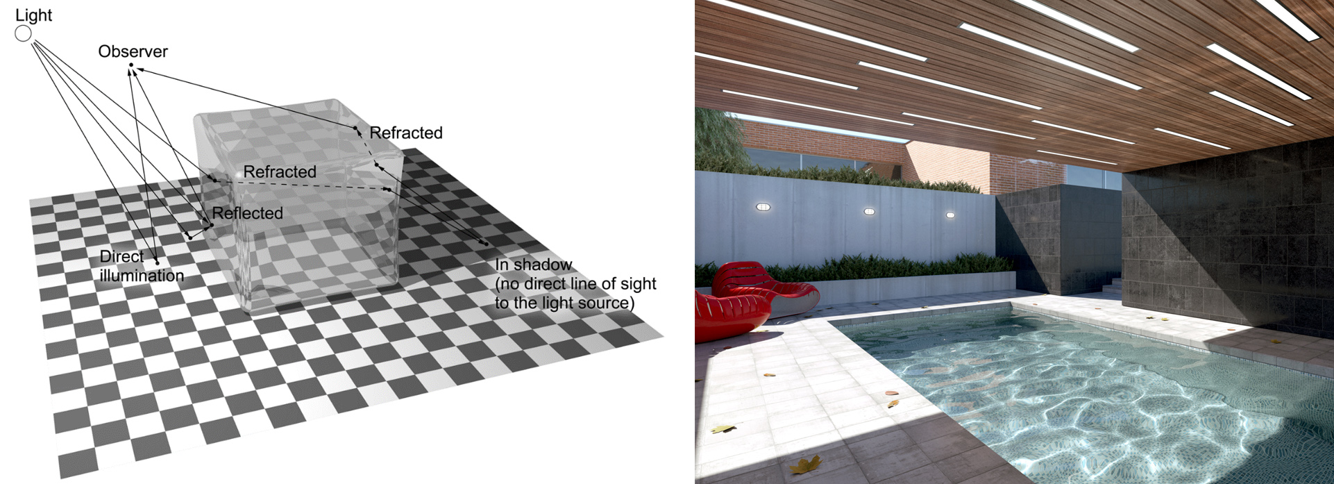
Stochastic Path Tracing
Stochastic path tracing is a method that generalizes the deterministic backwards ray tracing by statistically estimating the scattered energy at each hit point, indiscriminately taking into account all possible contributing directions, above or below th shaded point. Once primary rays have encountered a surface intersection, rays are spawned towards randomly chosen directions, which are deemed to have non-zero contribution, forming new path segments by recursively tracing the rays and encountering new surfaces. Light-emitting surfaces (light sources) can be randomly encountered this way, or they can be explicitly sampled by intentionally directing rays from the hot points towards them. The latter is called next event estimation and can greatly increase the convergence of the otherwise truly random process (see next figure).
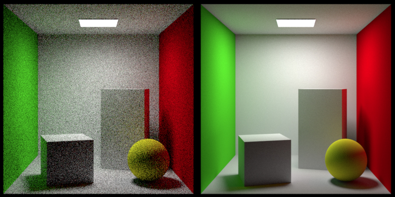
Rendering Equation. In essence, stochastic path tracing recursively estimates the integral of the rendering equation at each hit location. The rendering equation is one of the most fundamental equations in computer graphics as it describes the energy equilibrium at every surface location. Its extension to account for the energy scattering equilibrium at arbitrary locations in a medium is the volume rendering equation. The rendering equation can be described by the following formula:
is the outgoing radiance gathered from the hit point towards the query ray origin in direction . Directions here are all outgoing with respect to the hit point. So the ray that encountered the hit location had a direction . is the emitted radiance from the hit surface towards , if any. This term is zero for all but light-emitting surfaces (light sources).
The integral represents the sum of all possible contributions from any direction around point to the scattered light towards . How much light is scattered from each contributing incoming radiance is governed by two factors inside the integral: a) the BSDF (see appearance unit) and b) the flow of energy to the surface, as expressed by the cosine term. In the Whitted-style ray tracing algorithm, the integral of the rendering equation was replaced by sum of radiance from just two contributing directions: the ideal reflection direction and ideal transmission (refraction) direction .
Notice that radiance is included as both an input to and an output of the equation; the estimated outgoing radiance from one point is potentially the input to some other environment surface point. This is why the rendering equation cannot be computed analytically for all but the most trivial cases. It is a recursive form leading to the exploration of light-carrying paths through the environment, until the estimated contribution of radiance towards the virtual sensor pixels (through the primary rays) has converged to a result of satisfactory (low) variance.
Monte Carlo Integration. The core of the computational approach to evaluate the recursive rendering equation is Monte Carlo integration. In this statistical approach, the integral is estimated by approximating it by a discrete sum; samples of the integration parameter (here the incident direction ) are chosen within the integration interval (here the unit sphere of directions) based on a given distribution. Then for each sample the integrand is evaluated and the results are added.
Typically, if we have no hint about a "good" choice of a distribution according to which we should be drawing the samples, the uniform distribution is applied.
The Monte Carlo integral estimator converges to the expected value, which is the correct integral result, as the number of samples goes to infinity, provided that the sampling domain is completely covered by the sampling distribution. In this sense, we say that the method is unbiased and produces the correct visual outcome. However, since the estimator uses a finite number of samples, it introduces variance, which manifests as noise in the final result. Variance is greatly affected not only by the number of samples taken, but also by the quality of the "guesses" we make. To sample the integrand efficiently, i.e. generate samples and evaluate the function where it has a meaningful impact on the result, the distribution which we draw samples from needs to be proportional to the integrated function. This preferential sampling is called importance sampling and is key to achieving a high-quality result with a limited number of samples. However, since the integrand here contains the unknown inbound radiance , whose value will only be only available to us, after sampling the particular direction and recursively obtain radiance coming from another point or the background.
References
Historically, going back to the era of the REYES rendering architecture, a "fragment" corresponds to a primitive clipped at the pixel boundaries (Carpenter 1984), but nowadays we tend to use the term for the collection of primitive attributes resulting from the sampling (instead of dicing) of the primitive by the rasterizer.↩︎
Here transparency is used in a rudimentary manner, as a flat blending operation of see-through surfaces and content behind them and does not involve any physically-based light transport and refraction, although such a behavior can be approximated to some extent with multi-pass algorithms.↩︎
See Nanite technology by Epic Games: https://www.youtube.com/watch?v=eviSykqSUUw↩︎
Hierarchical occlusion culling: https://developer.nvidia.com/gpugems/gpugems2/part-i-geometric-complexity/chapter-6-hardware-occlusion-queries-made-useful↩︎
Entity component system https://en.wikipedia.org/wiki/Entity_component_system↩︎
For primitives with no area, such as line segments and points, we assume all points closer than a user-specified distance to the mathematical representation of the primitive to be "inside" or "on" the primitive.↩︎
Depending on pixel coverage.↩︎
B. Karis, R. Stubbe, G. Wihlidal. Nanite, a Deep Dive, ACM Siggraph presentation (advances in real-time rendering in games course), Epic Games, https://advances.realtimerendering.com/s2021/Karis_Nanite_SIGGRAPH_Advances_2021_final.pdf↩︎
Unless they hit the surface perpendicularly or there is no change of index od refraction.↩︎