The production of this online material was supported by the ATRIUM European Union project, under Grant Agreement n. 101132163 and is part of the DARIAH-Campus platform for learning resources for the digital humanities.

Preface
Audience
This introduction in computer graphics is intended for students with no computer science or mathematics background. Although the subject of computer graphics involves concepts and methodologies heavily riddled with and driven by mathematical tools, these notes follow an as descriptive approach as possible, in order to explain the basic principles of 2D/3D data representation, manipulation, processing and display, with an emphasis on practical examples and procedures. That said, a basic foundation of high-school-level mathematics is assumed, since it is sometimes impossible to precisely describe an operation or procedure, without resorting to the use of (simple) formulas and equations.
Objectives
The primary Objective of this material is to familiarize the interested audience with principles, concepts, technologies and practices related to the processing, manipulation and use of 3D content for the representation and visualization of digitized material, storytelling and interactive design. Where possible, it attempts to provide practical techniques, processing pipelines and examples for frequent tasks involving 3D content. It does not exhaustively cover the vast topic of computer graphics, nor does it act as scientific textbook. On the contrary, it attempts to concentrate on knowledge that is relevant to typical tasks of the intersection of digital humanities and computer graphics applications, providing some background that can help people outside the field, approach the computer graphics methods and tools with less apprehension and focus on the creative task at hand.
In terms of learning outcomes, after completing the online course, one will be able to:
understand basic algorithms and concepts of computer graphics. In turn this will enable one to:
understand how to work with software for the manipulation, modeling, editing and rendering of 3D content.
learn how to effectively process geometry in order to create 3D assets usable in popular software for 3D rendering and interactive presentation, or for archival and documentation purposes.
How to Cite this Work
This is not an AI-generated text, nor have any generative AI tools been used in the creation of the content presented. Therefore, although the entire course material is open and free to use, please cite the source, as an acknowledgment of the effort and time put in its creation:
Papaioannou, G. (2025). A Computer Graphics Primer for Humanists, online course, http://graphics.cs.aueb.gr
    @ONLINE {CGPrimer,
        author = "Georgios Papaioannou",
        title  = "A Computer Graphics Primer for Humanists",
        month  = "jun",
        year   = "2025",
        url    = "http://graphics.cs.aueb.gr"
    }
About the Author
Prof. Georgios Papaioannou is a Professor of Computer Graphics at the Department of Informatics of the Athens University of Economics and Business (AUEB) and head of the AUEB computer graphics group. He received a 4-year BSc in Computer Science in 1996 and a PhD degree in Computer Graphics and Shape Analysis in 2001, both from the National and Kapodestrian University of Athens, Greece. His research is focused on real-time computer graphics algorithms, photorealistic rendering, illumination-driven scene optimization and shape analysis. Since 1997, he has worked as a research fellow, developer and principal investigator in more than 20 research and development projects. From 2002 till 2007 he worked as a software engineer in virtual reality systems at the Foundation of the Hellenic World. Prof. Papaioannou has been the principal investigator for AUEB in many EU- and nationally-funded projects, as well as in R&D collaborations with the industrial sector. Personal website: http://graphics.cs.aueb.gr/users/gepap.
Preliminaries and Definitions
Introduction
Out of our five senses, we spend most resources to please our vision. The house we live in, the car we drive, even the person we love, are often chosen for their visual qualities. This is no coincidence since vision, being the sense with the highest information bandwidth, has given us more advance warning of approaching dangers, or exploitable opportunities, than any other.
Remark: Computer graphics harnesses the high information bandwidth of the human visual channel by digitally synthesizing and manipulating visual content; in this manner, information can be communicated to humans at a high rate.
Computer graphics encompass algorithms that generate (render) a raster image that can be depicted on a display device, using as input a collection of geometric and functional representations as well as procedural elements and their properties. These algorithms are based on principles from diverse fields, including geometry, mathematics, physics, and physiology.
In the same spirit, the aim of visualization is to exploit visual presentation in order to increase the human understanding of large data sets and the underlying physical phenomena or processes. Visualization algorithms are applied to large data sets and produce a visualization object that is typically a surface or a volume model. Graphics algorithms are then used to manipulate and display this model, enhancing our understanding of the original data set. Relationships between variables can thus be discovered and then validated experimentally or proven theoretically. At a high level of abstraction, we could say that visualization is a function that converts a generic data set to a displayable model.
Central to graphics is the concept of modeling, which encompasses techniques for the representation of graphical objects. These include surface models, such as the common polygonal mesh surfaces, smoothly-curved polynomial surfaces, and the elegant subdivision surfaces, as well as volume, implicit surface models and neural representations.
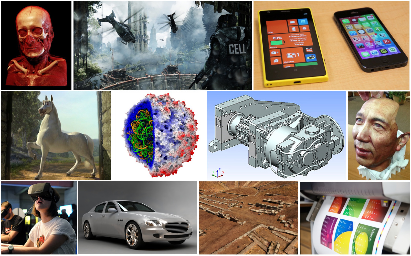
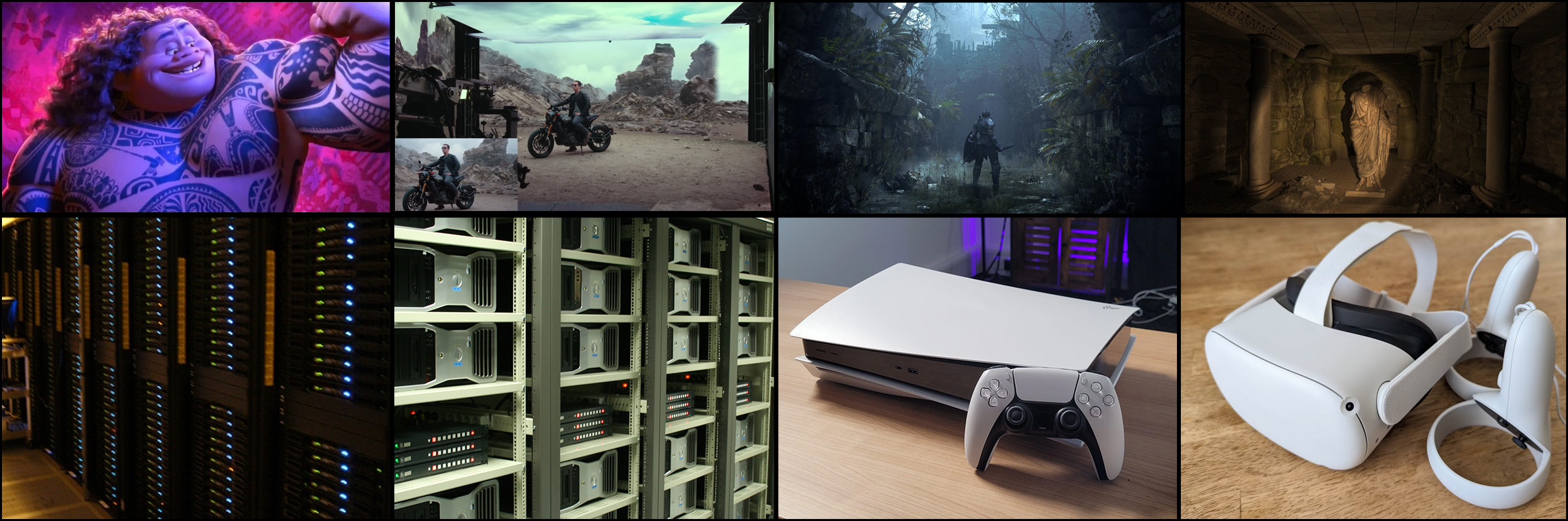
The applications of computer graphics are numerous and ubiquitous. Nowadays, computer games and interactive systems and software of all kinds constitute the main field of CG applications. In the last decades, computer games and interactive rendering drive the state of the art in high-efficiency algorithms and graphics hardware. Computer-Aided Design (CAD), Manufacturing (CAM) and Engineering (CAE) software systems use computer graphics for the physical product design using surface and solid modeling and geometric tools as well as the reverse engineering and simulation of physical objects and their properties.
Let us not forget that all graphical user interfaces (GUIs) rely on computer graphics methods for the display and manipulation of virtual controls and information, ranging from simple drawing tasks for the elementary GUIs of embedded controllers to the generation of elaborate effects for desktop and web graphics. Nowadays, all but the most basic of graphics-enabled devices use some form or another of hardware acceleration for the implementation of GUI rendering algorithms, mostly mapping the 2D display of interface graphics to the generic 3D rendering pipelines of modern Graphics Processing Units (GPUs).
The ability to create the impossible or non-existent, always brought computer-generated imagery (CGI) into the forefront of computational methods for the generation of special effects and fictional visuals for feature films. Although there does not appear to be a link between the use of CGI and box-office success, special effects and the integration of synthetic and filmed imagery are an integral part of current film and spot production. Films created entirely out of synthetic imagery are also abundant and most of them have met commercial success.
Direct human interaction and feedback poses severe demands on the performance of the combined simulation-visualization system. Applications such as flight simulation and virtual reality require efficient algorithms to generate convincing and immersive imagery that is fluently presented to the user, while maintaining immediate responsiveness of the overall system. The introduction of accessible commodity virtual hardware solutions has led to a boom in the use of stereoscopic rendering systems for high-quality real-time rendering of virtual worlds or the reproduction of precomputed or filmed videos. Augmented reality applications are becoming more and more sophisticated, integrating scene understanding and light field capture into a fused display of synthetic imagery and live view of the environment.
The investigation of relationships between variables of multidimensional data sets is greatly aided by visualization. Such data sets arise either out of experiments or measurements (acquired data), or from simulations (simulation data). They can be from fields that span medicine, earth and ocean sciences, physical sciences, finance, and even computer science itself.
Finally, 2D and 3D printing technology essentially use geometric representations, concepts and core computer graphics (display) algorithms to colorize, build or cut shapes and raster information as a physical output.
Definitions
Scenes and Virtual Environments
An aggregation of primitives or elementary drawing shapes, combined with specific rules and manipulation operations to construct meaningful entities, constitutes a three-dimensional scene. One or more 3D scenes constitute a virtual environment or virtual world. The two-dimensional counterpart of a 3D scene is a digital drawing or vector-based document.
The scene usually consists of multiple elementary models of individual objects that are typically collected from multiple sources and includes certain other components, such as virtual cameras and mathematical representations for materials and illumination sources, to dictate the way geometry should appear and be presented.
From a designer’s point of view, the various shapes contained in the scene or two-dimensional document are expressed in terms of a coordinate system that defines a modeling space (or “drawing” canvas in the case of 2D graphics) using a user-specified unit system. Think of this space as the desktop of a workbench in a carpenter’s workshop. The modeler creates one or more objects by combining various pieces together and shaping their form with tools. The various elements are set in the proper pose and location, trimmed, bent, or clustered together to form sub-objects of the final work. The pieces have different materials, which help give the result the desired look when properly lit. To take a snapshot of the finished work, the artist may clear the desktop of unwanted things, place a hand-drawn cardboard or canvas backdrop behind the finished arrangement of objects, turn on and adjust any number of lights that illuminate the desktop in a dramatic way, and finally find a good spot from which to shoot a picture of the scene. Note that the final output is a digital image, which defines an image space measured in and consisting of pixels. On the other hand, the objects depicted are first modeled in a three-dimensional object space and have objective measurements. The camera can be moved around the room to select a suitable viewing angle and zoom in or out of the subject to capture it in more or less detail.
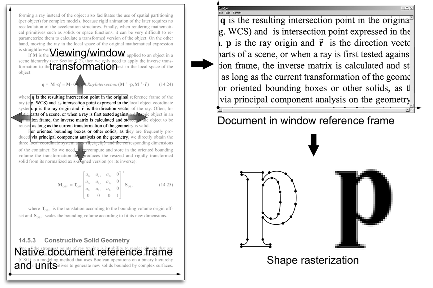
For two-dimensional drawings, think of a canvas where text, line drawings, and other shapes are arranged in specific locations by manipulating them on a plane or directly drawing curves on the canvas. Everything is expressed in the reference frame of the canvas, possibly in real-world units. We then need to display this mathematically defined document in a window, e.g., on our favorite word-processing or document-publishing application. What we define is a virtual window in the possibly infinite space of the document canvas. We then “capture” (render) the contents of the window into an image buffer by converting the transformed mathematical representations visible within the window to pixel intensities via rasterization, i.e. regular sampling on a grid (or raster).
As shown in the following figure, geometry and other elements, such as lights, action triggers, virtual cameras etc. can be hierarchically grouped together to form meaningful aggregate objects, which can help us better organize the virtual environment. This hierarchical organization is called a scene graph and can be beneficial both for the creator, to conceptually and ontologically cluster and reuse elements of the environment, and for the rendering system, as clustered entities can be collectively processed and displayed more efficiently. For example, a group of objects can be disabled for rendering as invisible or inactive, resulting in all included, dependent elements (this node’s "sub-tree") being inherently disabled as well. In the case presented in the figure, disabling the scene graph node "Dungeon" would result in also disabling all nodes stemming from it, i.e. the references to Part A, Part B and Part C.
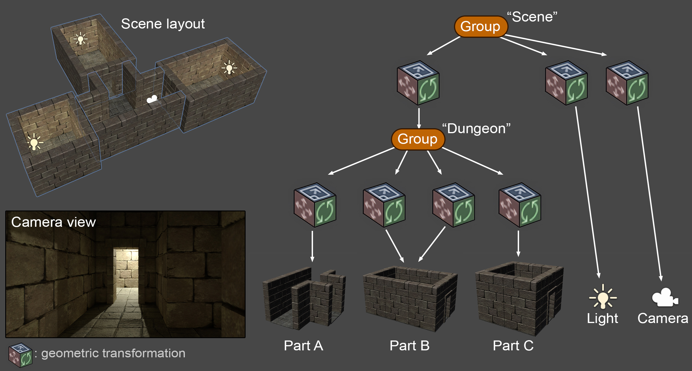
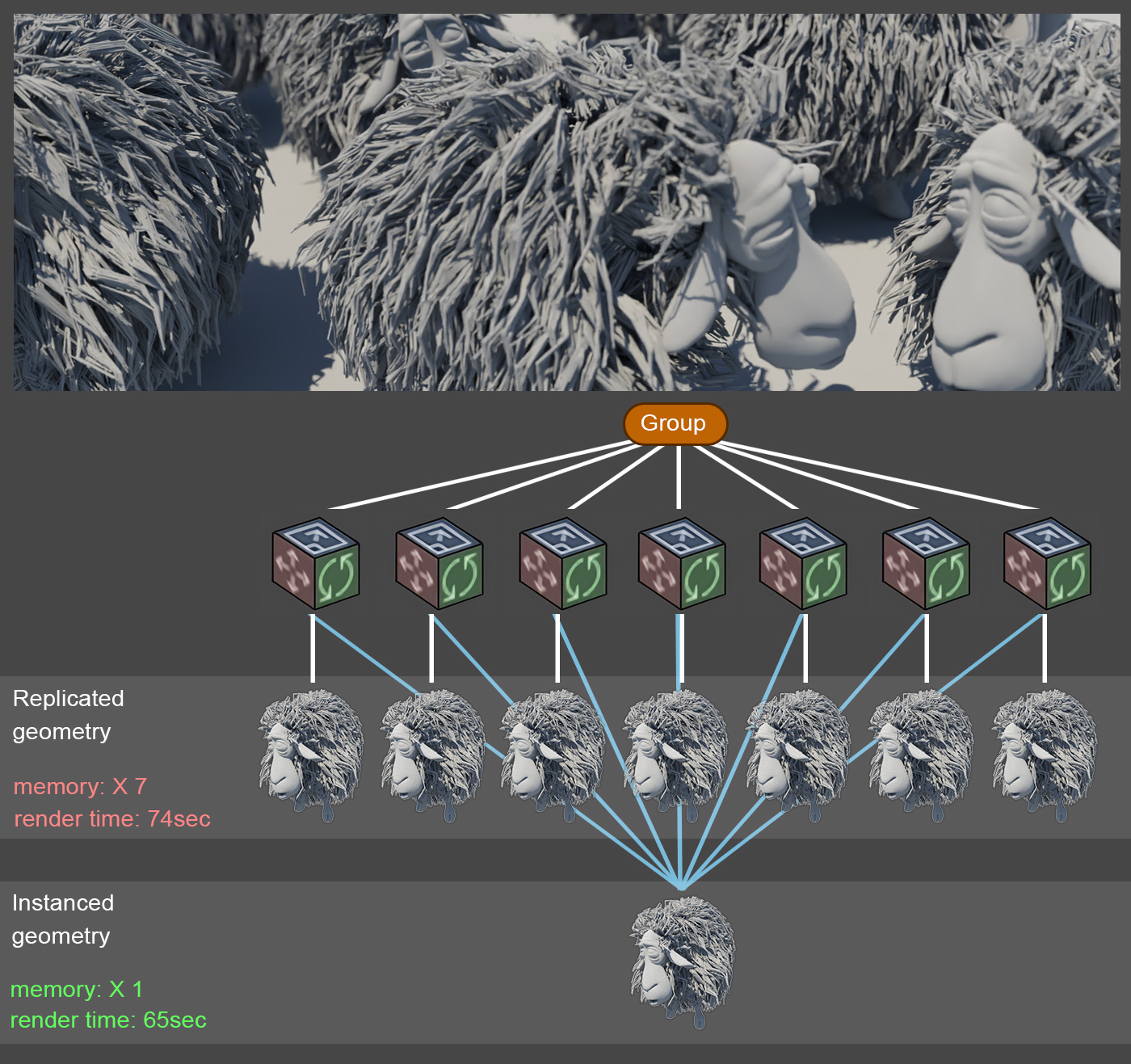
In a scene graph, geometry of identical objects does not need to be replicated, unless it must undergo a fundamental change in its topology or shape. It is beneficial both in terms of memory consumption and display performance to retain a single copy of the actual geometry and present it at a different size and pose by providing a distinct geometric transformation to each instance of the object. All instances internally reference the same geometric information, however, as shown in the figure below.
The objects can be models created in a 3D modeling software or 3D data acquired via 3D digitization. The basic building blocks of models are primitives, which are essentially mathematical representations of simple shapes such as points in space, lines, curves, polygons, mathematical solids, or implicit functions. However, geometric objects, along with their material properties can be represented in a more abstract manner, as is the case of Neural Radiance Fields (NeRFs) (Mildenhall et al. 2020).
To summarize, setting up a virtual scene corresponds to defining the following entities:
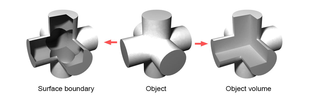
What to render: The geometry of the surface or volume of objects.
How objects are arranged The spatial relationships of geometric entities in three-dimensional space, i.e. the geometric transformations applied to the objects in the scene (including the cameras and light sources).
How objects look: The materials (substance qualities) and their finish that specify how energy (light here) interacts with the surfaces and volumes to render.
How objects are shaded: The energy (light) that is transmitted inside the virtual environment, illuminates the 3D geometry and is finally observed and recorded on the virtual camera, after being scattered on the surfaces or through the volume of objects. The lighting computations are done using a mathematical or statistical illumination model.
What are the dynamics of all the above: The temporal change (motion) of all the above parameters, including the intrinsic shape of objects (deformation). Animation can be predefined or determined at run-time via a simulation algorithm, user interaction or a combination thereof.
Rendering
Typically, a scene or drawing needs to be converted to a form suitable for digital output on a medium such as a computer display or printer. The majority of visual output devices are able to read, interpret, and produce output using a raster image as input. A raster image is a two-dimensional array of discrete picture elements (pixels) that represent intensity and color samples.
Rendering is the process of generating an image from a set of models (geometric representation) It is the final product of a general image synthesis task using a rendering pipeline.
Image synthesis includes many sub-tasks and algorithms for determining the proper coordinates of object primitives as these move in time, sampling the geometry and calculating the color of the samples using appearance properties ranging from simple drawing attributes to physically correct material properties, estimating the contribution of light to the shading of the surfaces and volumes and merging the results in the image buffer. Following chapters will focus on parts of the rendering process in more detail.
Rendering Pipeline
A rendering pipeline is a sequence of steps used to produce a digital image from geometric data.
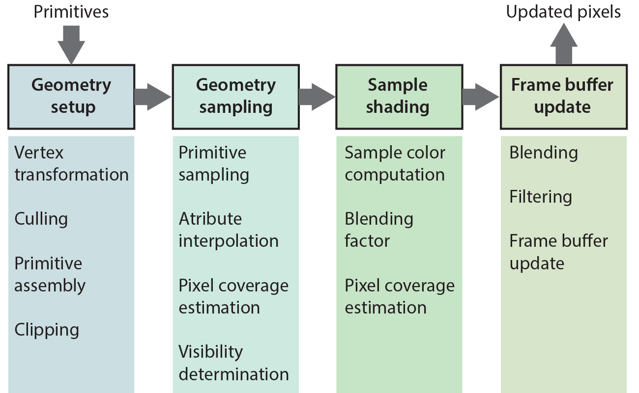
A high-level, conceptual overview of a rendering pipeline is presented in the figure below. Actual practical rendering pipelines such as the rasterization pipeline and the ray tracing paradigm can all be thought of as concrete instantiations of this abstract pipeline model. Furthermore, graphics pipelines, no matter how diverse, share many steps, concepts, mathematical models and tasks, such as geometric transformations, texturing, local sample shading, etc.
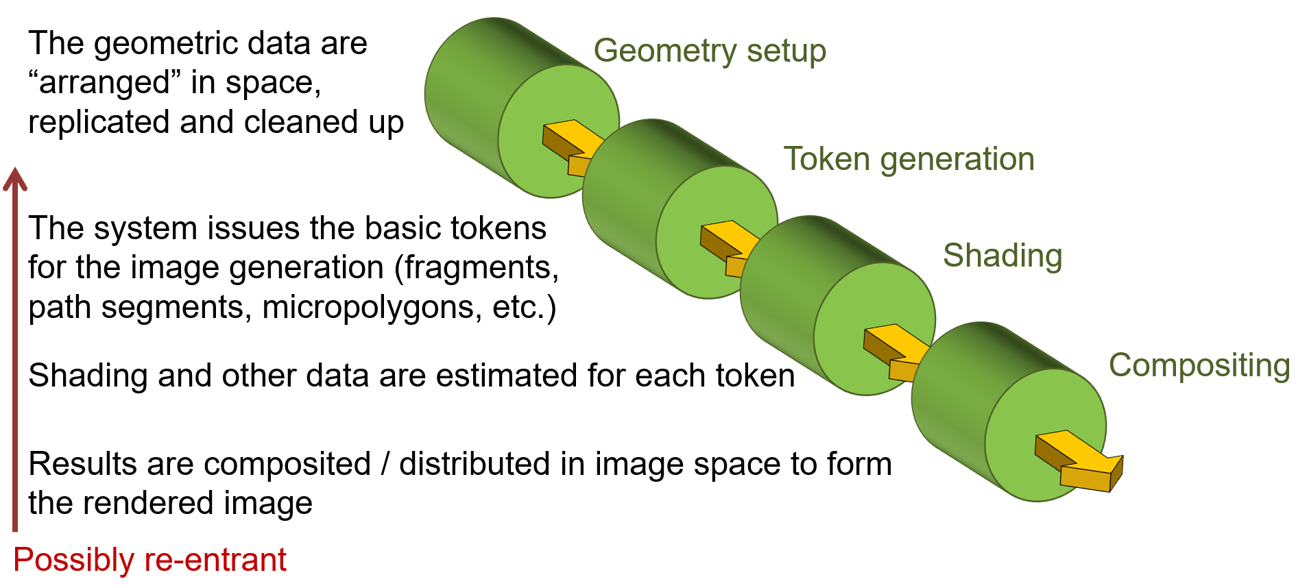
The first conceptual stage of a rendering pipeline regards all necessary geometric transformations and data manipulation that must be applied to a) bring the geometry to a shared coordinate system, b) gather all the geometric data and compute geometric properties required in the subsequent stages and c) compute any internal data structures, such as ray query acceleration data structures, primitive queues, etc. that will be needed for accessing and sampling the geometry. It is important here to note that operations in this stage affect the geometry at different levels. For instance, applying transformations such as rotation and scale to the geometry is done per vertex, if the content is a polygonal mesh, or per primitive, or object in other representations. Assembling and setting up triangle information for rasterization is done per primitive. Geometry culling is typically performed at object level. On the other hand, the construction of acceleration data structures for ray tracing is done both at object and primitive levels.
Next comes the sampling process, which is the core of the rendering pipeline and is usually a very intensive stage. For typical hardware rasterization pipelines, this involves the processing of each and every primitive emitted for rendering in order to create samples on them at (usually) a pixel-level granularity and the calculation of surface attributes from the primitive vertices (e.g. the 3 triangle vertices). For ray tracing, it corresponds to the generation and intersection of rays with the scene geometry and the determination of hit points on surfaces or volumetric samples, followed by a calculation of geometric and material attributes at these locations.
The shading stage determines the contribution of the sampled location, computed in the previous step, to the overall color of the corresponding image pixel. This is where materials and their spatiotemporal variation are taken into account and the light interaction with a surface or volume sample is computed, using a shading model. This can be as blunt and simple as assigning a single predefined color to the sample, or computing an elaborate photorealistic and physically correct scattering value for photometric light emitters. The resulting color is contributing to the synthesized image value of the affected corresponding pixel coordinate. Please note that the shading stage can be introducing additional sampling tasks, as is the case with the path tracing algorithm, which traces new rays and gathers the illumination contribution of other scene locations to the current point before applying the shading model and determining an excitant light value.
Finally, the compositing stage determines how the color from a single pixel sample affects and updates the image buffer. For example, in rasterization, this can be a simple blending operation that merges incoming results with the preexisting values in the image. For more complex pipelines, it can involve weighting operations on multiple results and stochastic re-sampling, thus re-entering the pipeline.
Below, a high-level overview of the ubiquitous hardware-implemented rasterization pipeline is presented. It is easy to map the high-level processes to the generic conceptual model of a rendering pipeline, as described above.
The Frame Buffer
During the generation of a synthetic image, the calculated pixel colors are stored in an image buffer, the frame buffer, which has been pre-allocated in the main memory or the graphics hardware, depending on the application and rendering algorithm. The frame buffer’s name reflects the fact that it holds the current "frame" of an animation sequence in direct analogy to a film frame. In the case of realtime graphics systems, the frame buffer is the area of graphics memory where all pixel color information is accumulated before being driven to the graphics output, which needs constant update. In the latter case, the need for the frame buffer arises from two facts: First, the popular process of image generation via rasterization is primitive-driven, as we will discuss in more detail in the rendering unit, rather than image-driven (as in the case of ray tracing) and therefore there is no guarantee that pixels will be sequentially produced. The frame buffer is randomly accessed for writing by the rasterization algorithm and sequentially read for output to a stream or the display device. So pixel data are pooled in the frame buffer, which acts as an interface between the random write and sequential read operations. Second, the image generation rate cannot always be synchronized with the image consumption rate by the output device, as it can finish earlier or later than what is expected by the output circuitry.
Interactive vs Offline Rendering
Offline rendering refers to the task of image generation, where visual quality in terms of detail, lighting and precision are not negotiable. The resources used for the formation of an image (or a frame of an animation) are only bound by budget constraints and time to render a single image is not critical. Results should be of high clarity and noise free and may take anything from several seconds to hours to complete the contents of a frame buffer. The term “offline” does not only refer to the non-interactive frame rate of the image generation but also to the fact that the resulting image is not ready for display, but rather a part of usually more complex production pipeline, involving several image compositing and post processing steps. Offline rendering is done on desktop workstations and distributed systems (rendering farms).
On the other end of the scale lies real-time rendering, where time to render an image is not negotiable, sacrificing visual quality, detail and accuracy to maintain a high frame rate. Responsiveness to interaction and smooth dynamic motion are the primary goals, resulting in a time budget to generate an image typically between 13 and 50 milliseconds (72 and 20 frames per second, respectively). The sacrifice in image quality can be manifested as noise, loss of geometric detail, simplification of animation, visual effects and lighting and the use of precomputed quantities instead of dynamically updated ones, where tolerable. Real-time rendering is important to interactive applications running on anything from a mobile device to a desktop system or games console.
The border between offline and real-time rendering is today significantly blurred, as graphics processing units become more and more powerful, while algorithms and graphics pipelines used exclusively in offline rendering in the past begin to deliver visuals at interactive frame rates. Real-time rendering, exploiting pre-processed lighting to a large extend, is used for responsive virtual filming sets, where the background is produced and updated on the fly on massive display panels. Photorealistic simulations can be run interactively and hybrid rendering pipelines and advanced hardware-assisted up-scaling and de-noising functionality help close the fidelity gap between the offline and real-time rendering world.
Hidden Surface Elimination
In computer graphics, relying on the specific order to draw graphics on a two-dimensional canvas resembles a painter’s algorithm: Farthest primitives are drawn first and successive, closer "layers", replace and cover the overlapping areas. This specific drawing order is often enforced in two-dimensional graphics and graphical user interface rendering tasks. However, this depth ordering is seldom available — let alone computable — in 3D graphics, since the order in which objects and primitives are provided for rendering is generally considered arbitrary and primitives may overlap at a scale that is finer than the primitive level. Typically ordering needs to be resolved at a pixel sample level.

Hidden surface elimination is the process of determining the correct order of overlap of a number of surface samples so that they are presented in a consistent and correct order when rendered.
Numerous hidden surface elimination algorithms have been proposed, some of which are specific to a rendering pipeline. A prominent example is the Z-buffer algorithm, which is tightly coupled with the rasterization concept and pipeline (see Rendering unit for more details).
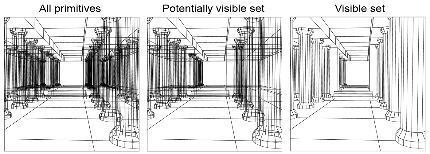
In some cases, hidden surface elimination is assisted by a more high-level procedure that can precede an accurate depth-sorting stage, which is the determination of the potentially visible surface set, as shown in the figure below. In this stage, we can discard parts of the geometry that are definitely not going to appear in the image, usually because their are either off-view or definitely obscured by other elements.
The Digital Image
The typical data structure for storing a digital image is a contiguous two-dimensional array (either row-major or column-major layout) in memory, the image buffer. Actually, every array in computer memory or file storage is a one-dimensional sequential arrangement, regardless of the dimensionality of the array. For example, an two-dimensional array of real numbers can be stored as consecutive segments of real numbers. Each cell of the buffer encodes the colour of the respective pixel in the image. The colour representation of each pixel (see Color chapter) can be monochromatic (e.g. grey-scale), multi-channel colour (e.g. red/green/blue), or paletted. When storing the image data in computer memory, for an image of pixels, the size of the image buffer is at least bytes, where is the number of bits used to encode and store the colour of each pixel. This number is often called the colour depth of the image buffer. When storing an image in a file, the data are typically divided into two segments, a header, containing information about the image metrics (dimensions, density, colour profile data, compression method, data layout etc.) as well as the data segment, where the actual image information is sequentially provided as a stream of bytes.
For monochromatic images, usually one or two bytes are stored for each pixel, which map quantized intensity to non-negative integer values. For example, an 8 grey-scale image quantizes intensity in 256 discrete levels, 0 being the lowest intensity and 255 the highest.
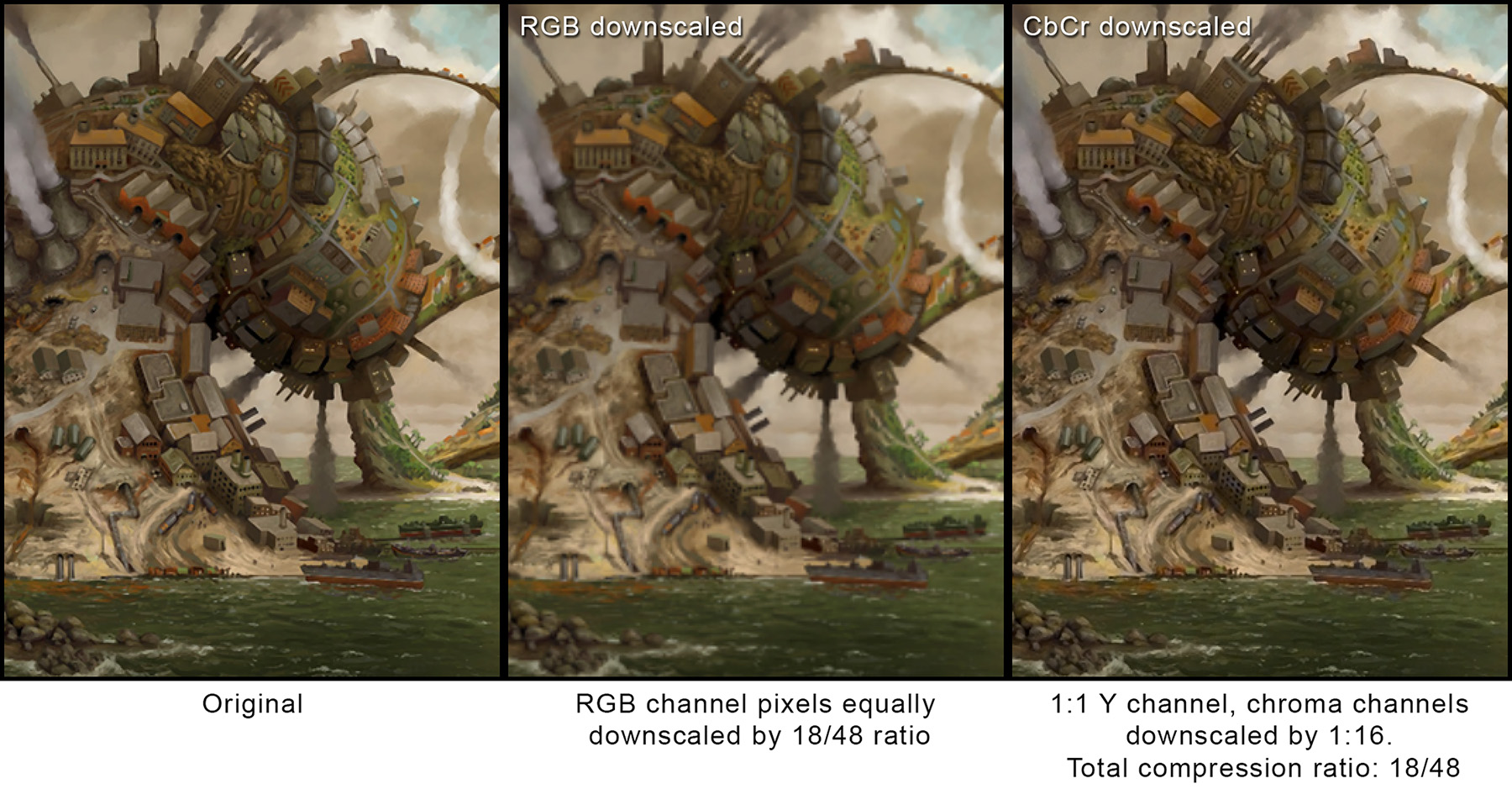
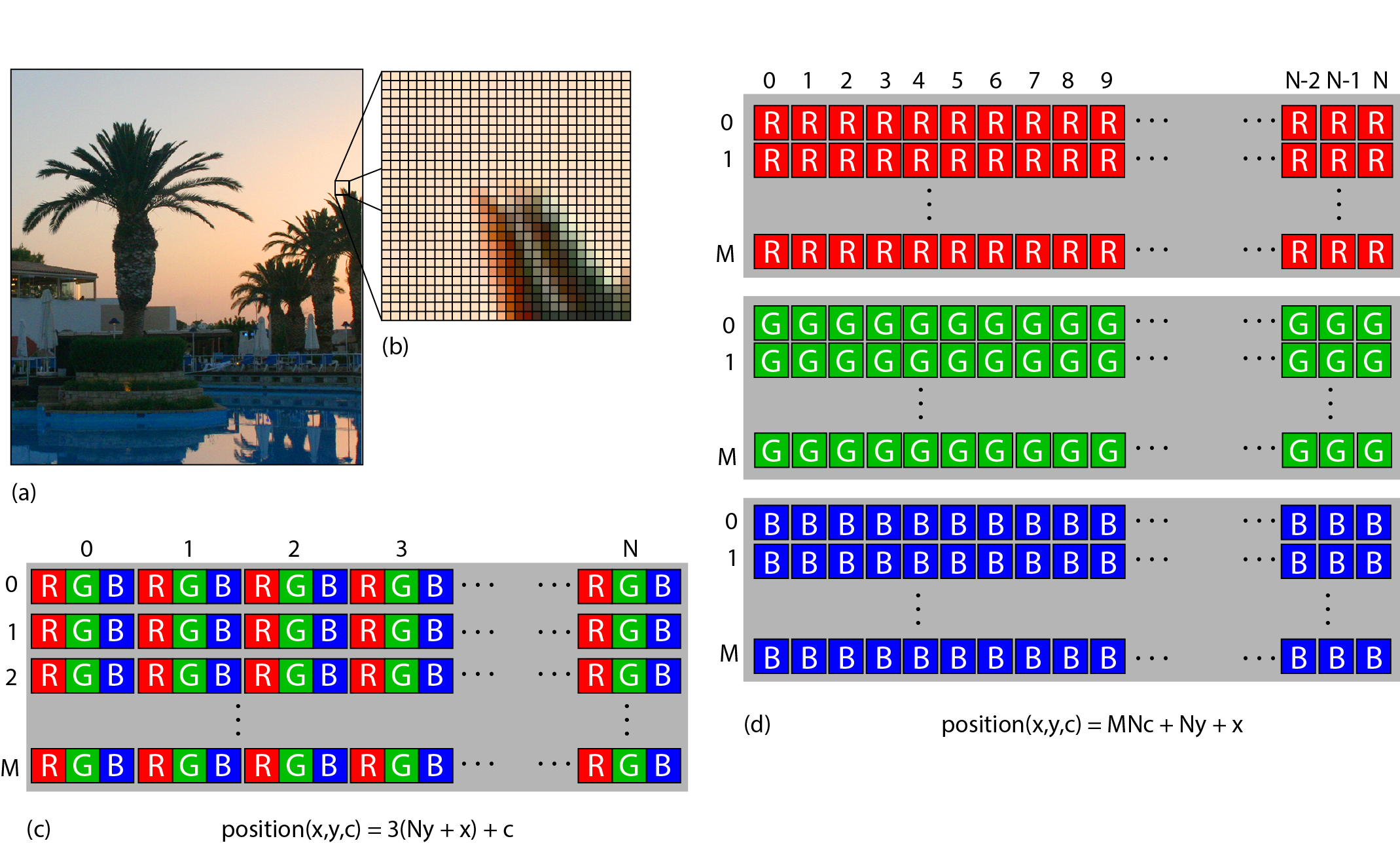
In multi-channel colour images, a similar encoding to the monochromatic case is used for each of the components that comprise the colour information. Typically, colour values in image buffers are represented by three channels, e.g. red, green and blue. For colour images, typical colour depths for integer representation are 24 and 48 . The colour components of a pixel are typically laid out in two arrangements for both file and in-memory storage: interleaved or in colour planes. In the first, the colour channels for a specific pixel are packed together one after the other in memory, forming an interleaved pattern. In the example of inset (c) in the following figure, the RGB data of an image are stored this way, forming a sequence of (RGB)(RGB)...(RGB) colour triplets in memory. In the alternative schema, the colour plane arrangement, individual colour components for the entire image are packed together one after the other, as shown in inset (d). There are merits for using either option as well as more intricate alternative storage patterns, such as the ones used for storing image textures in GPU memory. For operations on the image that perform calculations on all colour components of a pixel at once (e.g. grey-scale colour average) the interleaved mode is preferable as the data needed are close in memory (remember an image array is a big sequence of bytes) and therefore more likely to be in the processor cache. On the other hand, when applying an image filter on the colour channels separately (e.g. smoothing or median filters), arranging the colour values in planes ensures faster access to neighbouring values across different colours.
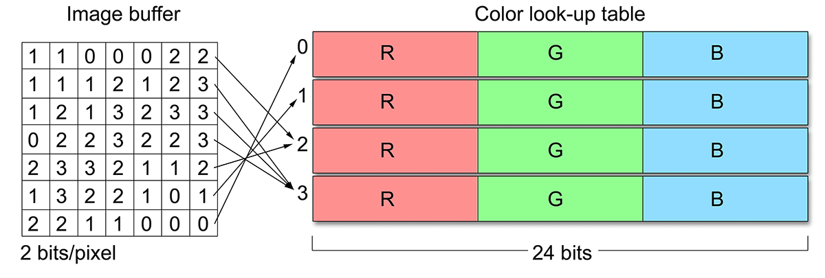
The above image representations are often referred to as true-colour, a name that reflects the fact that full colour intensity information is actually stored for each pixel. In paletted or indexed mode, the value at each cell of the image buffer does not directly represent the intensity of the image or the colour components at that location. Instead, an index is stored to an external colour look-up table (CLUT), also called a palette. An important benefit of using a paletted image is that the bits per pixel do not affect the accuracy of the displayed colour, but only the number of different colour values that can be simultaneously assigned to pixels. The palette entries may be true-colour values themselves. A typical example is the image buffer of the Graphics Interchange Format (GIF), a common format used for small-sized web assets, which uses 8 for colour indexing and 24-bit palette entries (see next figure). Another useful property of a palette representation is that pixel colours can be quickly changed for an arbitrarily large image. Nevertheless, true-colour images are usually preferred for image representation and processing, in general; integer formats offer simultaneous colours (large look-up tables are impractical) and image formats using floating-point (real) numbers only limit the values being represented by the numerical accuracy of the floating point convention employed. True colour data are of course also easier and faster to address and manipulate, since no de-referencing of the CLUT is necessary.
Common Image Formats
File formats for image data storage can be categorized in various ways, but their main characteristics that define their capabilities and storage requirements are the following:
Colour Channel Numerical Format. Most widely-used image file formats store the per-channel information of every pixel as an integer, typically as a single byte, i.e 256 levels per channel. JPEG and PNG are tyical examples of this strategy. Formats used in content generation and processing, digitization and medical imaging valso support floating point numbers, usually 16 bit or 32 bit long. The Tagged Image File Format (TIFF) and the Truevision Targa (TGA) formats are common formats that support floating point arithmetic representation for intensity values. Black and white encoders, such as the ones used for text document scanning (and fax transmission) employ binary encoding, as they are only interested in registering two states: bright and dark.
Number of Channels. Most image formats support multiple numbers of (colour) channels per pixel, but usually they include 1 (monochromatic), 3 (e.g. RGB) or 4 (CMYK or RGBA, A representing the transparency of an image layer). Some image formats do not support 4-channel configurations, such as the JPEG format.
Compression. Most file formats offer one form or of data compression or another. It is important to note however that compression can be either lossless or lossy, the latter resulting in degradation of the intensity information in order to more aggressively reduce the size of the resulting byte stream. JPEG, the most popular format in digital photography and image transmission and exchange uses a lossy compression method. This means that although the compression performed is perceptually friendly (the degradation will be very noticeable only at high compression levels), the format is not suitable for the storage of precision-sensitive invormation, such as normal maps (see Texture chapter) or the generation of digital surrogates. On the other hand, other formats, such as the TIFF format, may perform lossless compression (typically run-length encoding), making them suitable for such a task.
Colour Profile. Color profiles are important to reproduce the colour information stored in the image format as faithfully as possible across different media and display screens. They are used for the colour conversion between devices with different colour responses. It is therefore important to include the necessary device-dependent profile of the capture system in or alongside the file format. Some file formats dictate a specific colour profile (implied, e.g. sRGB), other embed the colour profile in the file format (e.g. JPEG), while some do not support the concept at all.
Image Metrics. Most formats used today provide fields in their header information for the density of the samples in the horizontal and vertical axis, usually in the form of a dots per inch (DPI) count. The density of the two axes is recorded separately, as certain devices like flat-bed scanners have a different stepping in each direction. Common file formats like JPEG and TIFF keep track of these measurements. DPI measurements have no physical meaning or usefulness for digital photographs.
In some formats such as the TIFF and the Adobe Photoshop file format (PSD), the image description also supports multiple layers and embedded non-image representations, such as vector graphics. In a similar manner, many document storage formats such as the widely-used Portable Document Format (PDF) and the Encapsulated Postscript (EPS) may include digital images encapsulated in their complex internal structure, along with text, vector drawings, colour profiles and layer information.
Remark: What format is appropriate for me? In computer graphics, image assets are used a lot to describe the texture of a surface or the appearance of widget or game sprite. Surface properties such as base colour, can use a typical JPEG format (with lossy compression), while other attributes can produce visible artifacts, when their values are drawn from texture images with lossy compression, such as reflectance and roughness maps. Image synthesis results are better stored in a high-precision integer or floating point format (EXR, TIFF, TGA) so that their exposure can be post-processed. For sprites and other on-screen entities that need to appear "perforated" and see-through, a file format that supports an opacity channel is useful (PNG, TIFF), so that this information needs not be saved in a separate file.
Compression
Today a vital part of the storage and transmission of data, is not a novelty introduced in the digital world. It pre-existed in analog communications for decades, as it was required for the efficient information broadcast in the noisy, low-bandwidth communications of the analog world. Compression can be lossless or lossy and the efficiency of a compression scheme is measured by its compression ratio: the size of the data after compression divided by the original size. In lossless compression techniques, the original form of the digitized data can be recovered in a bit-accurate manner, while a lossy compression scheme trades the introduction of some error for improved compression ratio.
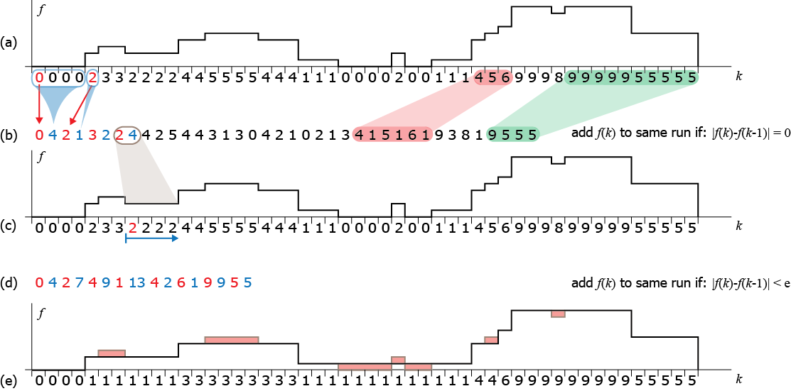
A simple example of lossless and lossy compression is shown in the following figure. A one-dimensional signal is compressed using a well-known lossless scheme: runlength encoding (RLE): consecutive identical values are replaced in the encoded sequence with the value and the number of times the value is encountered (b). This form of encoding significantly compresses runs of flat values (shown in green in (a)) but is very inefficient for highly variable data. Still, on average, it effectively reduces the size of most signals. The recovery of the original signal is straightforward as we only have to repeat a value to the output of the decoder as many times as explicitly recorded in the encoded sequence (c). Comparing the original and decoded signals (a and c) we can easily observe that RLE is a lossless compression method. To increase its compression efficiency, in (d) we allowed for some error to be introduced in the encoding process: instead of accepting only identical values in the current run that is being identified and encoded, we also accept values that differ less than an error margin (here 2) from the run value. As a result, longer sequences are converted to contiguous runs and tightly encoded. However, the decoded signal (e) has lost the corresponding variations and differs from the original.
Graphics Hardware
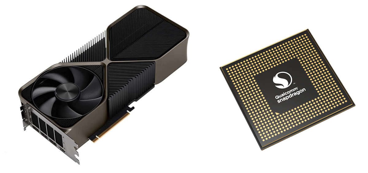
All computer systems that need to output raster graphics read color values that correspond to the visible dots on the display surface. The source of the output image is the frame buffer, which is sequentially read by a video output circuit in synchrony with the refresh of the output device. This minimum functionality is provided by the graphics subsystem of the host computing system, which may be included in a separate board, the graphics card. In many cases, multiple graphics boards may be hosted on the same computing system to drive multiple display terminals or distribute the graphics processing load for the generation of a single image. In other cases, e.g. in mobile and generally low-power devices, the graphics co-processors are integrated and fused into the central processing unit. This design option allows for a more efficient communication between host CPU and the graphics subsystem, but sacrifices scalability.
Image Generation Hardware
The early (raster) graphics subsystems consisted of two main components, the frame buffer memory and addressing circuitry and the output circuit. They were not unreasonably called display adapters; their sole purpose was to pool the randomly and asynchronously written pixels by the host computer in the frame buffer and adapt the resulting digital image signal to a synchronous serial analog signal that was used to drive the display terminals. The CPU performed the rasterization and randomly accessed the frame buffer to write the calculated pixel values. On the other side of the frame buffer, a special circuit, the digital-to-analog converter was responsible for reading the frame buffer line by line and producing the appropriate output voltage to drive the display. For modern digital displays, both integrated into the host device (e.g. mobile phones) or external, the digital-to-analog conversion step has become obsolete, as digital to analog conversion happens within the driver circuitry ofthe panels themselves.
In all cases, the output circuit operates in a synchronous manner to provide timed signaling for the constant update of the output devices.
The display refresh rate is the frequency at which the output display performs a complete redisplay of the whole image and it is synchronized with the rate at which image data are read from the output frame buffer of the graphics subsystem. It is measured in Hertz units (Hz), i.e. update cycles per second.
The frame refresh rate is determined by an internal clock and is set to a value mutually supported by both the graphics image generation hardware and the display device. It is typically set to standard values like 60, 70, 72, 75, 90 or 120 Hz.
In order to be able to decouple the rate and access pattern with which the display must be updated from the rate and random memory access with which the host system and the graphics subsystem generate a new frame, the idea of double buffering was born; a second frame buffer is allocated and the write and read operations are performed separately in the two memory areas, thus completely decoupling the two processes. When buffer 1 is active for writing (this frame buffer is called the back buffer, because it is the one that is hidden, i.e. not currently displayed), the output is sequentially read from buffer 2 (front buffer). When the write operation has been terminated for the current frame, the roles of the two buffers are interchanged, i.e. data in buffer 2 are overwritten by the graphics processing unit and pixels in buffer 1 are fed to the display output. This procedure is called buffer swapping.
Modern graphics processing units (GPUs) are massively parallel processing units with dedicated circuitry for performing primitive and texture image sampling, polygon clipping, hidden surface elimination and vertex attribute interpolation, compression, decompression and encoding and other intensive and frequent computations. A key element to the success of the hardware acceleration was the full implementation of the rasterization pipeline, where primitive and sample processing and shading is executed in a highly parallel manner and geometry processing, rasterization and texturing units have multiple parallel stages. However, modern GPUs also implement other specialized operations that are not rasterization-oriented, such as ray-triangle intersection queries for performing ray tracing efficiently and neural processing tensor cores.
Initial implementations of 3D acceleration hardware mapped the rasterization-based graphics pipeline for direct rendering into hardware, but the individual stages and algorithms for the various operations on the primitives were fixed both in order of execution and in their implementation. As the need for greater realism in real-time graphics surpassed the capabilities of the standard hardware implementations, more flexibility was pursued in order to be able to execute custom operations on the primitives but also not lose the advantage of the high speed parallel processing of the graphics accelerators. In modern GPUs, both the fixed geometry processing and rasterization stages of their predecessors are replaced by small, specialized programs that are executed in the graphics processors and are called shader programs or simply shaders.
The massively parallel nature (and of course shear numbers of processing cores) of the GPUs, lead to their exploitation to perform generic computations, not related to the rendering of 3D graphics and to a genre of computing paradigms collectively called General Purpose GPU computing (or for short GPGPU). Inevitably, image manipulation and processing tasks were the first to harness the power of GPGPU computing, by implementing image operations (such as colour manipulation and spatial filtering) entirely on the GPU. Several commercial applications nowadays for editing and processing photographs, heavily exploit the GPU for many computations. Furthermore, GPUs are extensively utilized in machine learning tasks, especially using neural networks, but also in 3D digitization, where parallel computations in the GPU enable the interactive alignment of partial scans and tracking of the target objects.
Output Hardware
Display monitors are the most common type of output device. However, a variety of real-time as well as non-realtime and hard copy display devices operate on similar principles to produce visual output. More specifically, they all use a raster image. Display monitors, regardless of their technology, read the contents of the frame buffer (a raster image). Commodity printers, such as laser and inkjet printers, can prepare a raster image, which is then directly converted to dots on the printing surface. The rasterization of primitives, such font shapes, vectors and bitmaps, relies on the same steps and algorithms as 2D real-time graphics.
Display Devices
During the early 2000’s, the market of standard raster image display monitors made a transition from cathode ray tube technology to liquid crystal flat panels. There are other types of displays, suitable for more specialized types of data and applications, such as vector displays, lenticular auto-stereoscopic displays and volume (holographic) displays, but we focus on the most widely available types.
The first liquid crystal displays (LCDs) suffered from slow pixel intensity change response times, poor colour reproduction and low contrast. The invention and mass production of colour LCDs that overcame the above problems made LCD flat panel displays more attractive in many ways to the bulky CRT monitors. Today, their excellent geometric characteristics (no distortion), lightweight design and improved colour and brightness performance have made LCD monitors the dominant type of computer display.
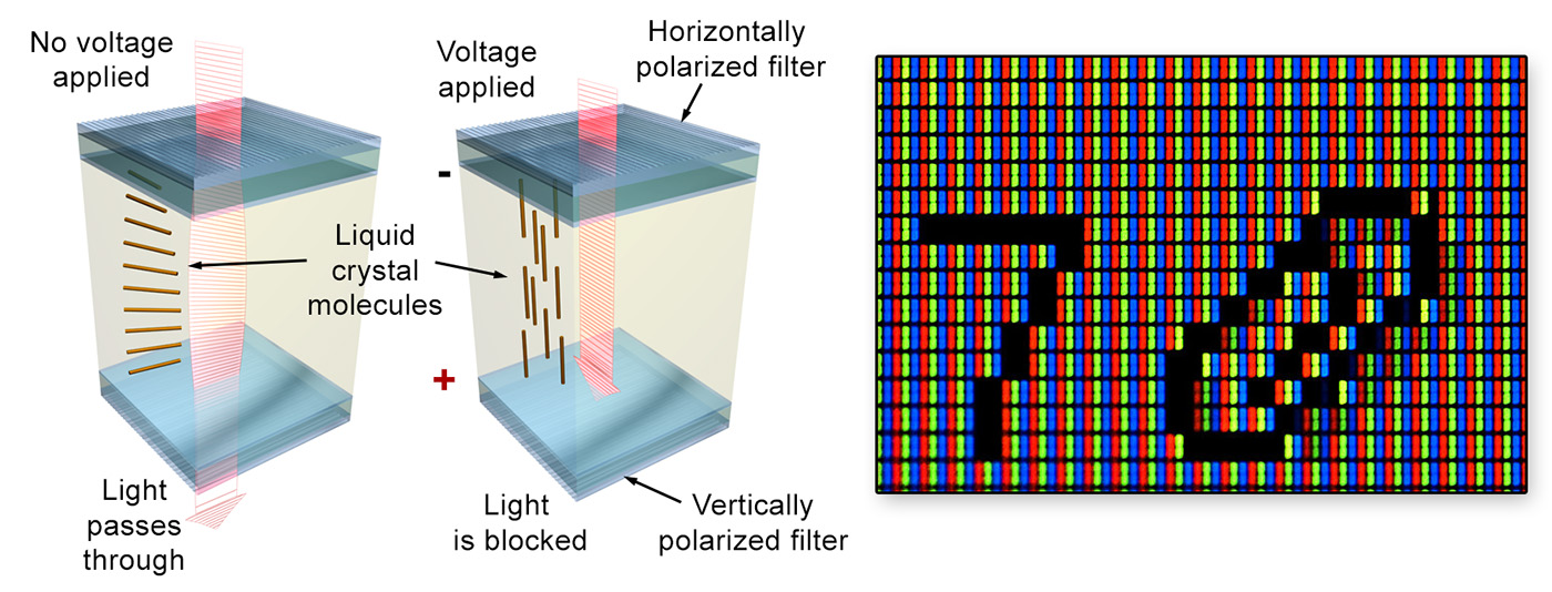
The basic twisted nematic (TN) LCD device consists of two parallel transparent electrodes that have been treated so that tiny parallel grooves form on their surface in perpendicular directions. The two electrode plates are also coated with linear polarizing filters with the same alignment as the grooves. Between the two transparent surfaces, the space is filled with liquid crystal, whose molecules naturally align themselves with the engraved (brushed) grooves of the plates. As the grooves on the two electrodes are perpendicular, the liquid crystal molecules form a helix between the two plates. In the absence of an external factor such as voltage, light entering from the one transparent plate is polarized and its polarization gradually changes as it follows the spiral alignment of the liquid crystal. Because the grooves on the second plate are aligned with its polarization direction, light passes through the plate and exits the liquid crystal. When voltage is applied to the electrodes, the liquid crystal molecules align themselves with the electric field and their spiraling arrangement is lost. Polarized light entering the first electrode hits the second filter with (almost) perpendicular polarization and is thus blocked, resulting in black colour. The higher the voltage applied, the more intense the blackening of the element is. LCD monitors consist of tightly packed arrays of liquid crystal tiles that comprise the ‘pixels’ of the display. Colour is achieved by packing 3 colour-coated elements close together. The matrix is back-lit and takes its maximum brightness when no voltage is applied to the tiles. TFT (thin-film transistor) LCDs constitute an improvement of the TN elements, offering higher contrast and significantly better response times, and are very frequently used in LCD flat panel displays. IPS (in-plane switching) LCD screens are a variation of the TN technology that offers a significant improvement in brightness and viewing angles. IPS technology is similar to the TN principle but the two electrodes are placed on the same side of the liquid crystal on one of the transparent layers and voltage aligns the LCD molecules parallel to the surface. The drawback of IPS displays is the relatively low refresh rate of the LCD panels, which make them somewhat less suitable for video editing and authoring applications and motion video production. However, IPS displays offer superior colour reproduction and colour constancy with respect to viewing angles.
For all the above LCD technologies, backlighting provides the active source of illumination. Nowadays, most display units use light emitting diodes (LEDs) for this purpose.The organic liquid crystal displays (OLED) offer an attractive alternative to TFT and IPS displays, especially for certain market niches like home entertainment and mobile devices, mostly due to the fact that they require no backlight illumination, have much lower power consumption and can be literally ‘printed’ on thin and flexible surfaces. An OLED display works without a backlight because it emits visible light itself, i.e. the material is electroluminescent. For this reason, it can display deep black levels, since there is no emission when not excited, and can be thinner and lighter than a liquid crystal display. In low ambient light conditions (such as a dark room), an OLED screen can achieve a higher contrast ratio than an LCD, making ideal for home cinema applications and sun-lit surfaces, such as mobile phones.
When choosing a display device, the following characteristics determine its suitability for a given task:
Resolution. Depending on the display surface size and viewing distance, a high-pixel-count, i.e. high-resolution panel may be necessary. Given a fixed display area size, increasing the displayable pixel count raises the planar pixel density. On the other hand, the human visual system has a maximum angular detail discrimination limit, which makes impossible to discern fine details of a certain frequency and beyond. The closer the display surface is to our eyes, the wider the footprint of a fixed number of pixels is on our retina and more detail we can distinguish. This of course also means that we can see the discrete pixel boundaries, an undesirable phenomenon called pixelization. Similarly, displaying content on very large display panels or projection screens requires very high resolutions, unless we can make certain the users or visitors are standing at a guaranteed minimum distance from the display surface.
Mobile devices and high-density desktop screens ar designed in such a way so as to be able to view content at a close distance. This in effect means that typical densities for such devices exceed 250dpi.
It is very easy to calculate the pixel density of a display screen; you divide the resolution along the horizontal and vertical dimensions with the corresponding physical dimensions of the display panel.
There are several ratings for the resolution of a display unit and the same holds for capture devices. One regards the total number of pixels on the surface of the display or sensor and is measured in MegaPixels (MPs or MPixels). Another rating corresponds to the horizontal or vertical resolution of an image. Common formats include the ""true" HD (high definition) or 1080p format that corresponds to an image with 1920 horizontal resolution and 1080 pixels vertical and therefore an aspect ration of 16:9. The next industry-standard format we often encounter is the UHD or Ultra High Definition, otherwise known as 4K resolution, the naming corresponding to the horizontal pixel count of the image: 3840 by 2160 pixels in total.
Refresh rate and response time. The refresh rates achievable by the circuitry of the display device are very critical for the display of animated content, such as videos or rendering of interactive applications. What is very important to note however is that sometimes the switching of the individual elements of the display panel from full brightness to darkness and vice versa may not be able to follow the refresh rate. This is particularly evident on IPS screens, resulting in ghosting when rapid illumination transitions occur on the spot.
Colour Gamut. This is the range of achievable colours by a certain device capable of reproducing different colour values. The wider the colour gamut or coverage of the colour gamut of the intended colour space for viewing or processing of content, the better. This is often a feature of display panels that is often neglected, when determining the suitability of one for a task. It is however of utmost importance for colour proofing and processing of digitized material, as improper colour mapping of digitized values to the display output can severely distort the perceived colour. High-quality and professional computer screens offer a good coverage of the sRGB colour space, the standard colour space for digital image manipulation and display tasks. The same does not hold for TV screens, which may sacrifice colour faithfulness for contrast, unnatural, vivid saturation or brightness.
Projection Systems
Digital video projectors are visual output devices capable of displaying real-time content on large surfaces. Two alternative methods exist for the projection of an image, rear projection and front projection. In rear-projection setups, the projector is positioned at the back of the display surface relative to the observer and emits light, which passes through the translucent material of the projection medium and illuminates its surface. In front-projection setups, the projector resides at the same side as the observer and illuminates a surface, which reflects light to the observer.
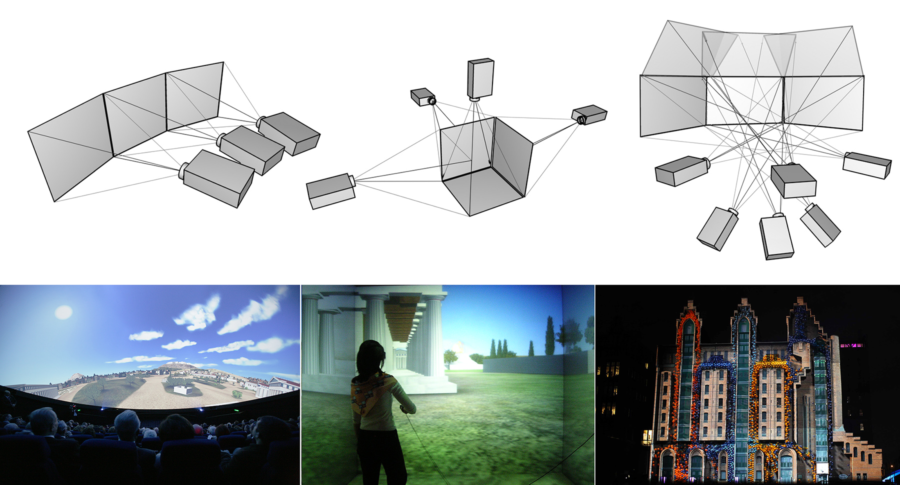
In exhibitions and museums, both technologies offer attractive advantages and are equally used. Back-projection systems are "invisible", as they can be seamlessly integrated into panelling, and their beams are not affected by visitors and other obstacles. On the other hand, front-projection systems offer much brighter images and can be easily configured in multiple projector setups to display content on large and curved surfaces and the floor, or be used for projection mapping, i.e. the art of exploiting the shape of real geometry to alter the illumination reflected off it using properly aligned projectors and suitable content.
There are two main projector operation principles. In the first, a beam of white light is split using dihroic mirrors into three primary color sub-beams that pass through LCD panels, which modulate their intensity over the image plane. the beams are then overlaid again and projected via a lens system. In the second type of projector, a high-intensity beam is directed on an array of reflective cells that modulate the incident light and reflect it to the lens system for projection. The widely used DLP projectors fall in this category, where micro-mirrors embedded on a silicon substrate are electrostatically flipped and act as shutters which either allow light to pass through the corresponding pixel or not. Due to the high speed of these devices, different intensities are achieved by rapidly flipping the mirrors and modulating the time interval that they remain shut. A more expensive technology, LCOS (Liquid Crystal on Silicon) modulates light by transparency over a reflective surface and offer higher contrast. All different technologies can take advantage of the three-way light splitting technique, to offer higher color fidelity. Due to the use of micro-mirrors, DLP projectors can be driven with higher intensity light sources, such as laser beams, to provide adequate illumination levels for use in outdoor environments or long distances.
Printing
The technology of electronic printing has undergone a series of major changes and many types of printers (such as dot-matrix and daisywheel printers) are almost obsolete today. The dominant mode of operation for printers is graphical, although all printers can also work as ‘line printers’, accepting a string of characters and printing raw text line by line. In graphics mode, a raster image is prepared that represents a printed page or a smaller portion of it, which is then buffered in the printer’s memory and is finally converted to dots on the printing medium.
The generation of the raster image can take place either in the computing system or inside the printer itself, depending on its capabilities. The raster image corresponds to the dot pattern that will be printed. Apart from the dynamic update of the content, an important difference between the image generated by a display monitor and the one that is printed is that colour intensity on monitors is modulated in an analog fashion by changing an electric signal. A single displayed pixel can be ‘lit’ at a wide range of intensities. On the other hand, ink is either deposited on the paper or other medium or not (although some technologies do offer a limited control of the ink quantity that represents a single dot).
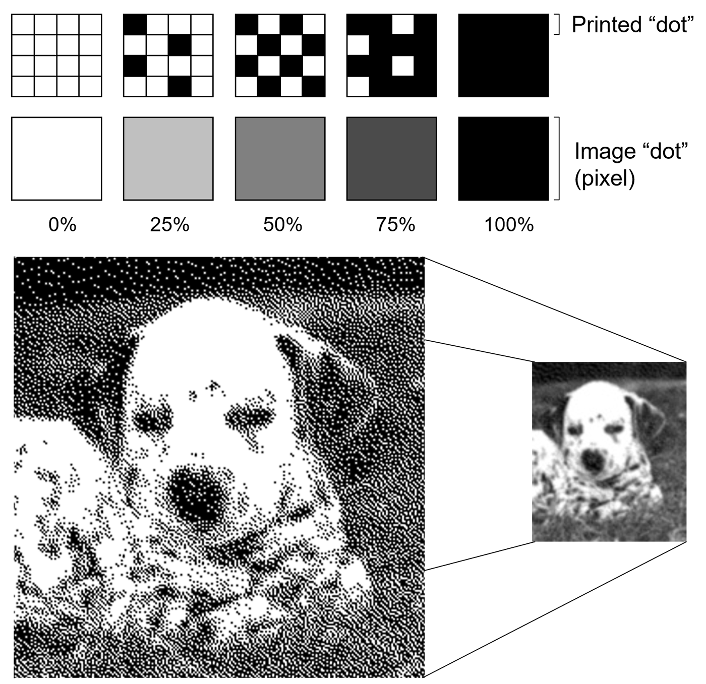
Half toning To achieve the impression of different shades of a colour, the technique known as half-toning is used. Pixels of different intensity can be printed as patterns of coloured dots from a small selection of colour inks, by varying the density of the dots and to a certain degree their size. When observed from a typical distance, the human visual system blurs the dots together, making them appear a continuous gradient of shades.
Remark: It is crucial to understand that the dot density (dots per inch — DPI) advertised for a printing device is not directly related to the image resolution of the document that is sent for printing, unless the the latter is purely black and white. Due to the half-toning process, a single digital image pixel corresponds to multiple printed dots. In simple terms, printing an image of a certain resolution (say 300dpi) on printer with the same dot density will result in a printed image of far less discernible detail for non-extreme shades than the original.
The two dominant printing technologies today are inkjet and laser. Inkjet printers form small droplets of ink on the printing medium by releasing ink through a set of nozzles. The flow of droplets is controlled either by heating or by the piezoelectric phenomenon. The low cost of inkjet printers, their ability to use multiple colour inks (usually 4-7) to form the printed pixel colour variations (resulting in high quality photographic printing) and the acceptable quality in linear drawings and text made them ideal for home and small office use. On the other hand, the high cost per page (due to the short life of the ink cartridges) their low printing speed and low accuracy make them inappropriate for demanding printing tasks, where laser printers are preferable.
Laser printers operate on the following principle: a photosensitive drum is first electrostatically charged. Then, with the help of a mechanism of moving mirrors and lenses, a low-power laser diode reverses the charge on the parts of each line that correspond to the dots to be printed. The process is repeated while the drum rotates. The ‘written’ surface of the drum is exposed to the toner, which is a very fine powder of coloured or black particles. The toner is charged with the same electric polarity as the drum, so the charged dust is attracted and deposited on the drum areas with reversed charge and repelled by the rest. The paper or other medium is charged opposite to the toner and rolled over the drum, causing the particles to be transferred to its surface. In order for the fine particles of the toner to remain on the printed medium, the printed area is subjected to intense heating, which fuses the particles with the printing medium. Colour printing is achieved by adding three more (colour) toners and repeating the process three times. The high accuracy of the laser beam ensures high accuracy linear drawings and halftone renderings. Printing speed is also superior to that of the inkjet printers and toners last far longer than the ink cartridges of the inkjet devices. A variation of the laser printer is the light-emitting diode (LED) printer: a dense row of fixed LEDs shines on the drum instead of a moving laser head, while the rest of the mechanism remains identical.
Dye-sublimation (or dye-diffusion) printers rely on a heating process to mix dyes onto a specially coated paper, producing a continuous tone print. Along with high-end inkjet printers, they constitute today the primary printing devices for photographs. Some dye-sublimation printers use CMYO (Cyan Magenta Yellow Overcoating) colours, a system that differs from the more recognized CMYK colour set in that the black is eliminated in favour of a clear overcoating. This overcoating is also stored on the ribbon and is effectively a thin layer which protects the print from discolouration from UV light and the air, while also rendering the print water-resistant. During the printing cycle, the printer rollers will move the medium and one of the coloured panels together under a thermal printing head, which is usually the same width as the shorter dimension of the print medium1. Tiny heating elements on the head change temperature rapidly, laying different amounts of dye depending on the amount of heat applied. Some of the dye diffuses into the printing medium.
3D Printing
3D printing has revolutionized many aspects of fabrication and prototyping, by allowing the quick preview and testing of parts, the easy fabrication of difficult to build objects as single pieces, and the inexpensive fabrication of objects in small quantities. For this reason, aside from industrial applications, 3D printers have found their way to niche application domains, such as fabrication of surgical implants, dentistry, art and cultural heritage.
In order to print a 3D model, special processing by dedicated software is required to slice the model into layers and compute its internal structure. The typical input is the 3D polygonal mesh of the object to print, typically in STL or OBJ format. It is good to provide "watertight" 3D models, i.e. models that have been pre-processed by either some modelling software (like Blender or 3D Studio MAX) or 3D digitization software and contain no open surfaces, self-intersections, holes or other degeneracies. The slicing pre-processor can typically handle open surfaces, but may result in inferior printing quality, if not taken care of, prior to this stage.
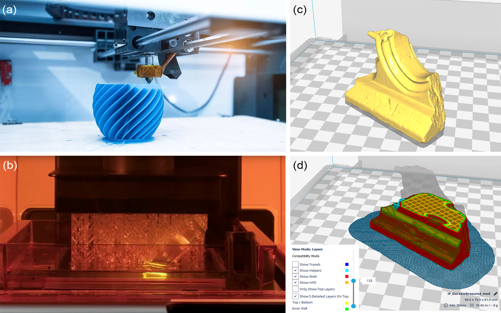
3D printing is conducted in layers and the two most popular techniques are "Fused Deposition Modeling" (FDM) and "Stereolithography Additive Manufacturing" (SLA). The first uses a filament made of thermoplastic or other material that is fed to an extrusion nozzle which melts it and controls its flow on or off. The printing head bearing the nozzle can be moved with numerically controlled stepper motors relative to the printed model so that it can deposit the molten material, in a similar fashion as milling machines or plotters work. The object is produced by extruding melted material to form layers as the material hardens immediately after extrusion from the nozzle. This technology is most widely used with two plastic filament material types: ABS (Acrylonitrile Butadiene Styrene) and PLA (Polylactic acid). Consumer-grade FDM 3D printers develop the model on a flat horizontal plate, which can be moved on the vertical axis. The printing head moves on the plane, depositing layers. SLA 3D printers are equipped with a tank filled with a liquid resin. At the bottom of the tank, there is a UV light emitting high-resolution LCD, which instantly cures a layer of resin, according to the displayed pattern of the currently printed layer. An extruder mechanism pulls upwards the already cured parts of the model and new layers are deposited at the bottom.
As typically 3D printers operate by depositing layers of material along one axis, the slicing software samples the 3D model in thin slices and exports the trajectories that the printing head must follow to imprint the outlines of each layer over the already deposited material so far. To make possible the printing of dangling parts with respect to the printing direction and also strengthen the internal structure of the object, the underlying algorithm inserts additional supports both on the exterior and the interior of the object. All the surplus material has to be manually scraped off the object after it is produced and its surface may require chemical or mechanical treatment to achieve a smoother result, depending on the printing technology used and the density at which the object was made.
Digitization
The process of digitization aims to represent an object, image, sound, document or, formally, any analog signal by generating a series of numbers that describe a discrete set of its samples. By the term analog, we define a signal that is represented in a continuous way, i.e. we can obtain a value for it at any given point of its input domain. Conversely, in digital signals, values are discrete and only a finite set of values per input domain unit are captured. The values of the samples are also digital, i.e. they are converted to an arithmetic representation of finite precision, which typically means that not all values can be represented, neither in terms of granularity nor range.
In theory, many data and signals that we encounter in the physical world have one form of intrinsic discontinuity, thus making them "non-continuous" by nature. However, for all practical purposes, the original form is considered an analog input, since "we can do no better" at representing its information. A typical example is the scanning of an old newspaper to obtain a digital image and put it in a news archive. The pictures in the newspaper are produced by a process called half-toning (see Color Representation chapter), which approximates a continuous image by black and white dots of variable density. This is definitely a discretized form of representation of the information depicted, however from our perspective, this is the original signal.
Digitization is the conversion of analog information in any form (text, photographs, voice, etc.) to digital form with suitable electronic devices (such as a scanner or specialized computer chips) so that the information can be processed, stored, and transmitted through digital circuits, equipment, and networks.
The output of the digitization process is a digital representation or digital form of the original signal. Typically, each sample in the digitized data is finally expressed in the form of binary numbers, i.e. numbers that can be represented with bistate or binary digits, either 0 or 1 (bits). Both integers and real numbers can be converted to a digital representation, using special conventions for their binary storage in the memory units and circuitry of a computing system. Decimal integers are directly converted to their binary counterparts and stored as such. Real numbers are split in a decimal and fractional part, which are separately encoded as binary numbers and stored with a fixed precision in each part, i.e. a fixed number of bits allocated to them. This kind of representation builds on the well-known scientific notation for real numbers, where a real number is expressed in an exponential way. For example: can be written as and can be written as . In these particular examples, the decimal point or radix has moved or floated so that all description digits are moved to the decimal part, while the exponent encodes the magnitude of the number. This floating-point representation allows us to represent both very small and very large numbers efficiently, using a fixed number of bits, with minimal loss of information.
Frequently digital representations are missing characteristics of the original, physical artefacts. Texture, smell, sound, tactile feel, other important attributes can likely never be truly copied. One interesting thing about this fact is the use of the word "important" here: it signifies our need for some specific sensory input in order to comprehend, analyse and semantically process information about the original. Still, in many cases this requirement is tied to the mental processing we humans perform or have been trained to apply in order to discriminate and classify input from our environment. Thinking in a purely task-driven manner, are we sure that going through the sensory channels of a human expert is the only way to interpret things? For instance, we use touch to feel the relief of a patch of textile to complement our visual information about it with data about its softness, elasticity, moisture etc. Have we ever thought whether this information is irrelevant to a computational system performing the same classification for us? What if electron spectroscopy, a method that humans cannot perform but a machine can, may reveal three times more information crucial for the recognition and categorization of the same original object? In other words, what is important information to capture and what is not, is subject to the processes the particular data are going to be used in. We are very often biased against digital methods because we are trained to work otherwise. Also, we often consider preservation for its own sake, rather than a task for safekeeping and advancing knowledge.
Digitization and Computer Graphics
Aside from the theoretical aspects of (2D/3D) digitization, which shares a considerable theoretical background with image synthesis tasks, especially for the geometric representation, processing and camera modelling part, the products of digitization are typically used as input to any number of general or specific computer graphics processes, from geometry analysis and synthesis to rendering and scientific visualization and their applications. Very frequently, photographs and other two-dimensional digital imaging data, 3D scans, captured motion and even conventional video are either directly used as items to be presented via computer graphics algorithms or are used as "assets" to synthesise visual representations of content to be displayed in image synthesis tasks.
When digitizing an object, we must understand that:
There is no perfect digital representation; you can always do better, given the proper effort and technology.
Therefore:
We are responsible of setting a quality level that is "good enough" for a task at hand: The loss of information due to the digitization process does not prevent the recovery of important information that characterizes the original artefact.
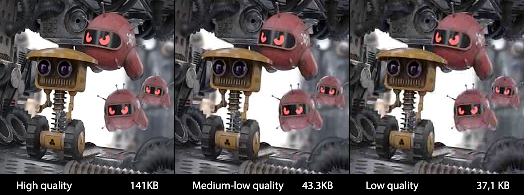
A 3D model’s geometric and textural detail, a scanned document, a digital photograph, can only be "good enough" for the specific purposes that the digital asset is going to be used for. For visualization purposes, not all captured detail is equally important. Digitization often results in very highly detailed models in terms of geometric representation. This excessive detail may or may not be relevant to the study or documentation of the original object, but it certainly poses severe problems when attempting to display geometric information, especially on medium- or low-end devices.
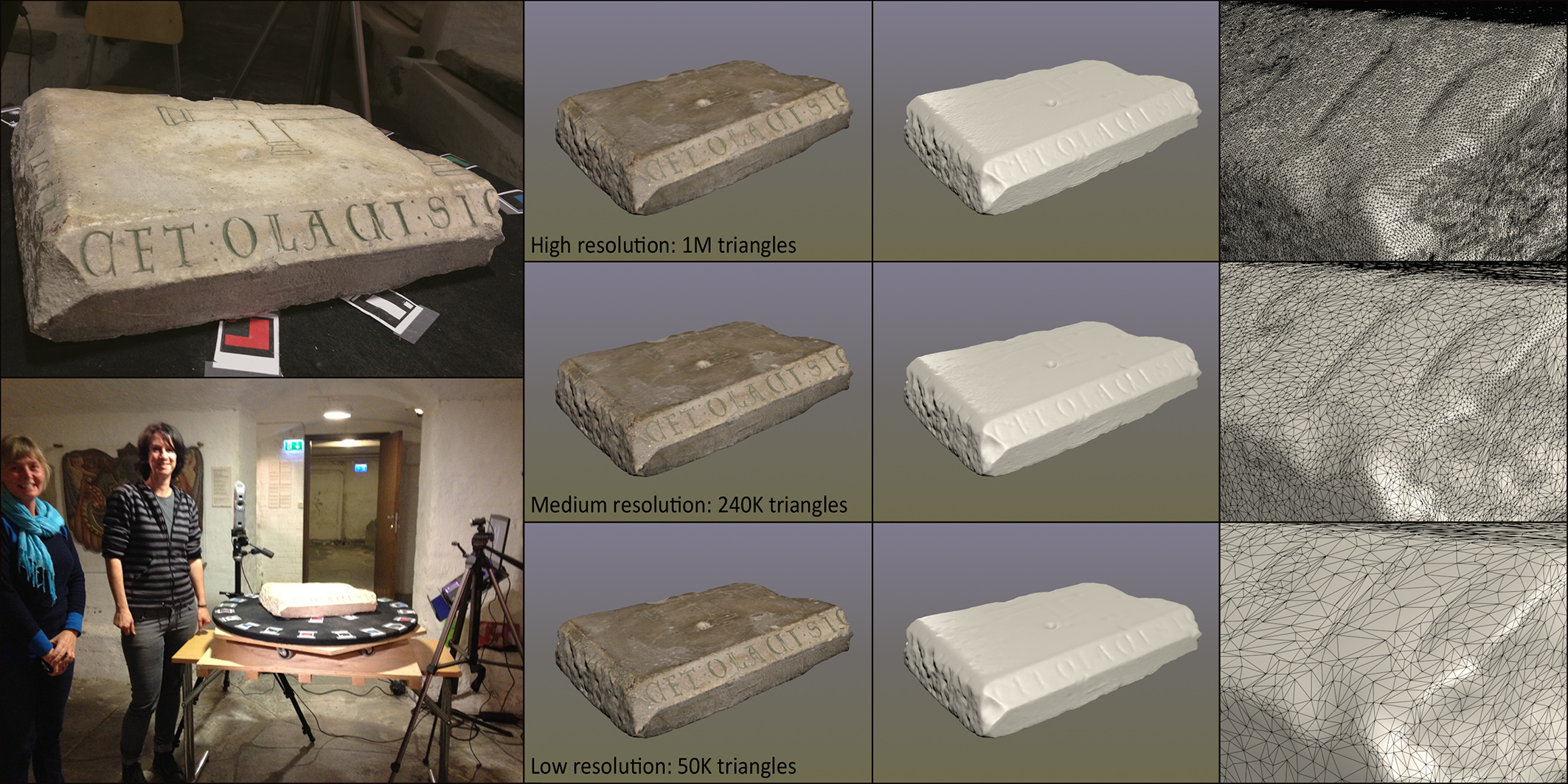
Typically we produce multiple versions of a digitized artefact, intended for different purposes. The example in the following figure demonstrates this: A high resolution version of a 3D scan is acquired and archived along with the raw input. Then the point cloud is reduced to obtain a more manageable volume of information for processing and computer-based analysis (medium resolution). Finally, the geometry is further reduced to get a low-resolution version of the model that is better-suited for display on low-end systems or the web.
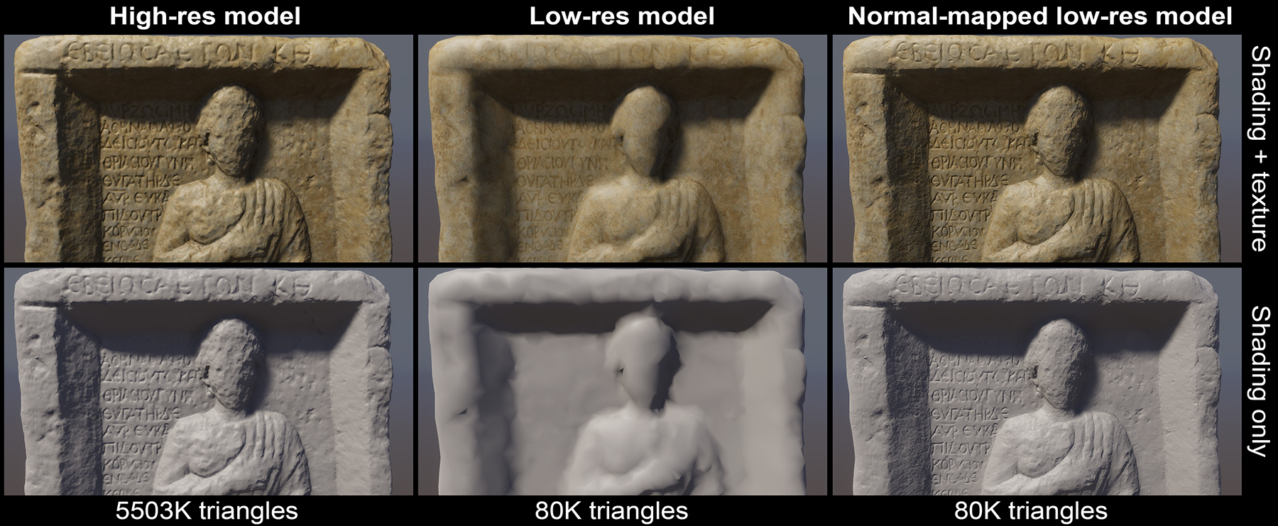
Furthermore, low-resolution 3D models can still visually represent their high-resolution counterparts, when established detail transfer techniques are exploited, such as normal "baking", which maps surface detail of the high-fidelity model as surface orientation texturing on the low-resolution one, as demonstrated in the figure below.
When digitizing three-dimensional objects, we must maintain a consistent and accurate scale between the dimensions of the original artefact and the digitized data. This in turn translates to two different requirements: a) the inclusion of a reference unit in the data format and b) for measurement methods that operate in relative scale, the inclusion of a physical reference object of known dimensions along with the target artefact and the digitization of both. The latter is very important in photography-based digitization methods, where the spatial parameters of the camera and lens systems are usually not pre-calibrated.
Sampling and Quantization
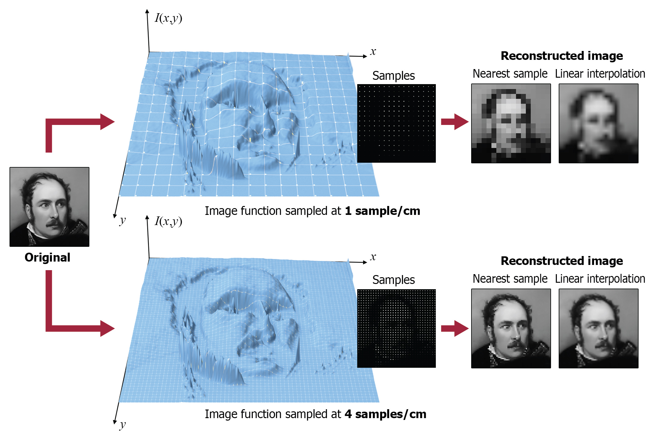
Digitization involves two processes, both of which can potentially degrade the original information: sampling and quantization. Sampling is the process of choosing discrete locations on the original signal and recording a reading (a sample value) at that location (see the marked sampling locations in the example below. Sample values at this stage are considered exact. For finite input signals (w.r.t. the frame of observation) the number of samples is finite and usually pre-determined. E.g. taking a photograph with a digital camera translates to sampling the field of view illuminating the sensor at a fixed (image) resolution. Other signals can be sampled indefinitely, e.g. temperatures at a weather station, creating an "infinite" series of samples. For both cases however, samples are drawn at regular intervals, i.e. using a certain period . The units and meaning of the period corresponds to the input domain that we are using. For example, when sampling an audio track, samples are drawn at a fixed time interval, while when scanning a document, we determine the horizontal and vertical spacing (period is in length units here) of the image samples. The density of the samples or the sampling rate determines the frequency at which we perform the digitization. In general, as the frequency corresponds to the number of samples per input domain interval unit (time, length etc.), ; the denser the sampling, the higher the frequency and smaller the sampling period. For example, scanning a document using 200 samples ("dots") per inch (dpi), results in a sampling period of 1/200 in and a frequency of 200 . For signals evolving in the temporal domain, the frequency of an event is measured in or Hertz (Hz). For the case of video sequences, where we have a succession of of still images or frames, the sampling rate is measured in frames per second (fps).
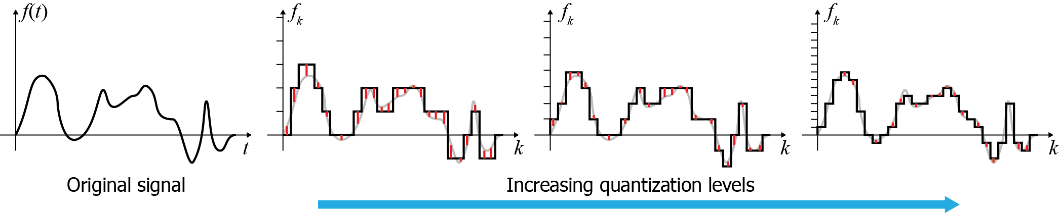
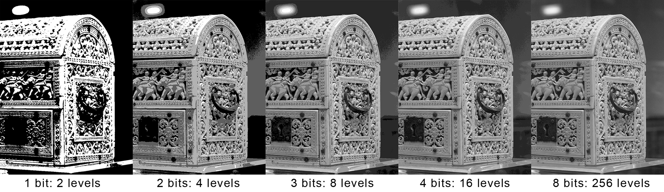
Samples are converted to the numerical representation available in the system performing the digitization. During this process, values are typically rounded to a fixed set of numbers (such as integer steps), a process known as quantization. Quantization in essence performs a discretization (although not always uniform) of the sample value scale, resulting in loss of information about intermediate values (quantization error). The next figure shows an example of the error introduced when quantizing the input values at different number of levels. Typical quantization processes in real systems allocate at least 256 levels (8 bits ) for the input value, with many applications using at least 16bit sample representation (65536 levels) or floating point numbers. It is worth noting that in many cases, due to the fact that the digitization process involves analog-to-digital conversion hardware, this too contributes to the error margin by the superposition of noise. This noise level makes the use of higher-precision quantization methods ineffective, since the noise has obscured the detail. Noise and other sources of intrinsic device error can also affect the sampling rate in various ways, imposing a maximum effective sampling rate in many applications.
In order to process, reproduce or randomly access (in the case of computer graphics digital assets) a digitized signal, sampled information must be interpreted as their continuous counterpart, by various approximation techniques. The mathematical counterpart to this process is the convolution of the sample sequence with a reconstruction filter that "spreads" the individual samples to fill in the missing (continuous) information between the sample locations. Digitized or digitally born assets may be re-sampled at a different rate to be used in a certain information processing task. In essence the reconstruction filter performs an interpolation of the discrete values and in practice, established interpolation functions such as constant, linear or cubic interpolators are employed.
Poor sampling of the original signal invariably leads to the phenomenon of aliasing.
Aliasing is the miss-interpretation of the samples as a different signal than the original during the reconstruction. This happens because not having enough samples to represent your signal means that more than one signals could actually pass through the (relatively sparse) recorded samples, as these leave room for uncertainty.
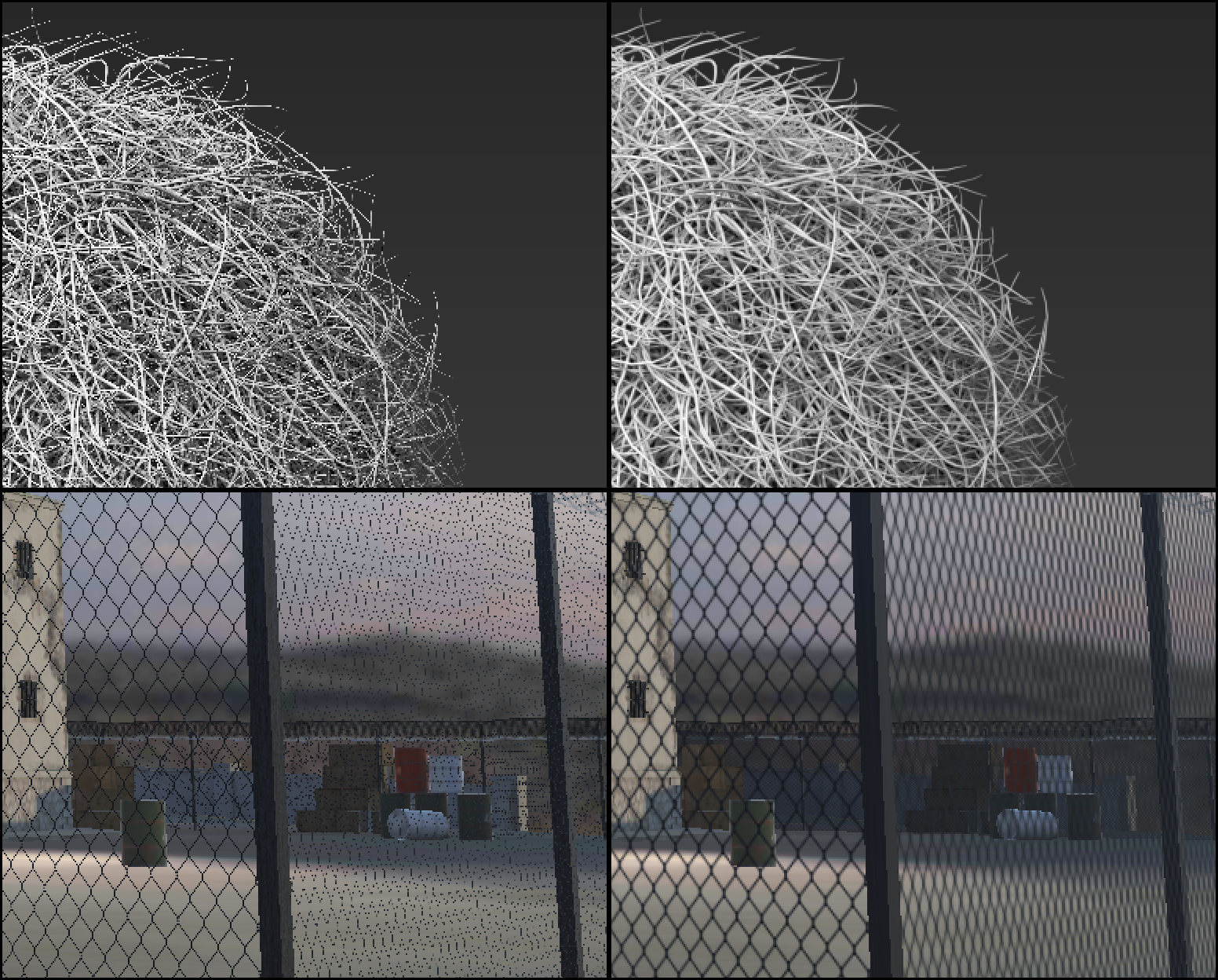
In computer graphics, aliasing is frequently manifested during image synthesis, when regularly sampling the image buffer domain (pixel-sized sampling period). Textural detail on surfaces or thin structures, with thickness or contrast variations smaller than 2 pixels, will be poorly represented by the raster image, resulting in noisy, temporally unstable patterns, often deviating significantly from the intended signal. Examples of the phenomenon are shown in the following figure.
Color
Color has always been used in art and studied for millennia. Today the study of color, and the way humans perceive it, is an important branch of physics, physiology, psychology, art as well as computer graphics and visualization. Understanding how humans interpret color, how to efficiently represent and store color information with minimal loss and how to reproduce the subtle tonal variations as faithfully as possible are all crucial factors for a successful digitization and presentation of visual content (T. Theoharis et al. 2008).
Color Perception
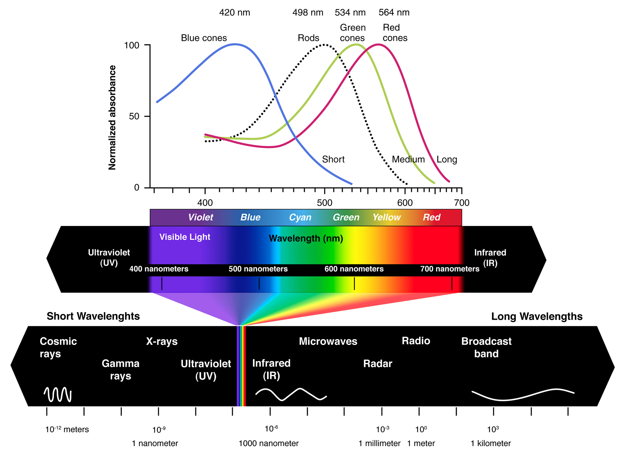
The human visual system consists of two functional parts, the eye and (part of the) brain. The brain does all of the complex image processing, while the eye functions as the biological equivalent of a camera (Maintz 2005). Light first crosses the cornea and the iris aperture, which act as a lens and a diaphragm respectively. and after travelling through the clear vitreous body inside the eye, reaches the retina, i.e. the inside of the eye ball surface where the photoreceptors are situated (see figure next). Similar to a camera diaphragm, the iris opens wide to allow more light to reach our photoreceptors under dark conditions, while it constricts in normal daylight. On the retina, the light rays are detected and converted to electrical signals. The human eye has two types of photoreceptors: rods and cones. Humans have three different cones, each having a greater response to a particular light wavelength, corresponding to blue, green and red colors. By combining the response of the three types of cones in a small area of the retina we are able to blend their signals to perceive any color. This process is called trichromacy. The combined range of our tri-stimulus vision is only a tiny part of the electromagnetic radiation detectable nowadays.
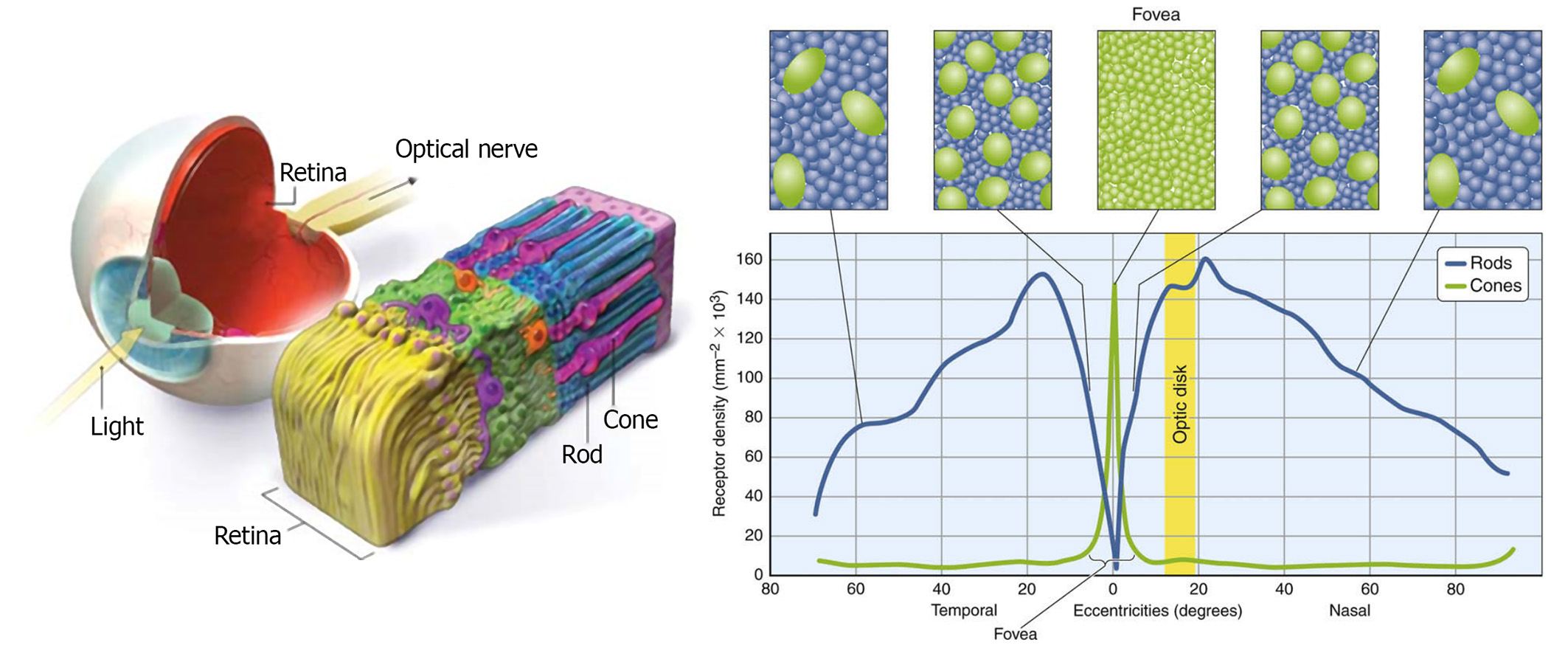
We encounter about 100 million rods in a human eye, with their population spread fairly evenly about the retina, except at the fovea, where there are almost none. Fewer cones (about 6 to 7 million) are mainly located around the fovea, but can be also found in a much lower density in the entire retina. No photoreceptors are found at the point where the optic nerve attaches to the eye (the so-called blind spot). With regard to the connectivity of rods and cones, an analysis of the neural circuitry of the human eye reveals a tendency of the photoreceptors to be connected with dedicated "lines" to the optic nerve, while moving to the periphery of the retina, photoreceptors tend to become aggregated. This is the primary reason why our visual acuity is higher in the fovea and also linked with the photopic vision, mostly due to the cones. The cumulative effect of all receptors combined is a frequency response mainly centerd at green hues, as shown in the next figure. This means that we can better discriminate shades of green and bluish green (after all we are descendants of a tree-dwelling species).
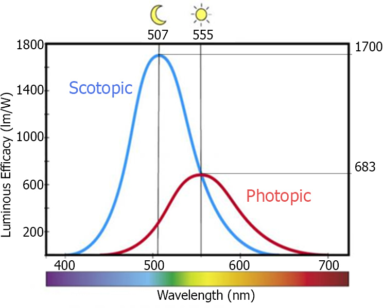
Non-linearity of Perception
The ability to detect a spot of light does not depend so much on the luminance of the spot itself as on the difference in luminance of spot and background, i.e., the local contrast. Of course, the luminance must be above some minimal value, but it is the contrast of spot and background that must be above a certain threshold before we can detect the spot. We call this threshold the just noticeable difference. Weber discovered that the just noticeable difference is proportional to the background luminance . In other words, the higher the background luminance, the higher the contrast needs to be before we detect a difference (Maintz 2005).
The just-noticeable difference between two stimuli is proportional to the magnitude of the stimuli.
These kinds of experiments have been performed in many different sensory modalities to measure our abilities to discriminate: intensities of 2 lights, intensities of two sounds, pressure on the skin, weight of two objects, intensity of electric shocks, and a whole host of other things. The result is always the same: The difference threshsold is proportional to the baseline/starting intensity. The generality of this observation proved so surprising that it has been called a psychological law, and it is named after its discoverer, Weber. Later, it was validated that the local contrast of a stimulus, i.e. its amplitude of variations versus the the local mean stimulus level, directly translates to increased neural activity in the brain. For us, this behaviour of responding to the stimulus levels has a very important consequence for color perception:
Remark: The retina is more sensitive at low light levels and less sensitive at high light levels: We distinguish more light levels at dark parts of an image.
This is summarized in the following diagram:
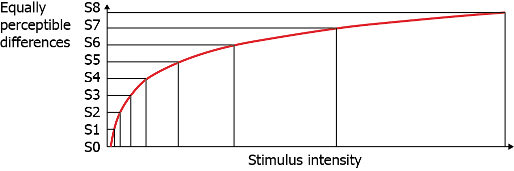
Psychology of Color Perception
After the trichromatic response is passed to opponent interpretation in the physiology of our optic systems, the final engagement of color perception occurs in our minds. This interaction complicates and potentially confounds our objective measurements, so it is critical to be aware of the typical issues that the filter of our mind brings to the arena of color perception.
Opponency. The input from the eyes’ tristimulus response is interpreted based on a mapping we perform from that input to a color space determined by three axes of opposing sensations. We define our color perception by identifying the perceived color based on its degree of greenness to redness, blueness to yellowness, and darkness to lightness.
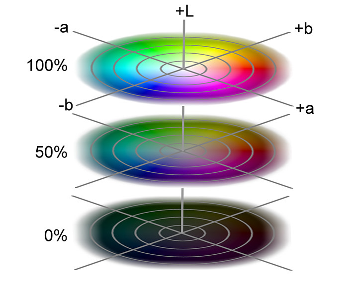
These three pairs of opposites — green-red, blue-yellow, dark-light — form an internal color basis for HVS to represent any color. These opponent color pairs form a basis in a mathematical sense, too, as they are exclusive color entities, occupying opposing ends of the range of our interpretation and thus are linearly independent.
Color Constancy. Color constancy is how our mind adjusts our color perception to discount or remove the effects of an overall color cast due to a colored illuminant. If we see someone wearing a yellow sweater illuminated by a bluish cast of light, we still ‘see’ a yellow sweater, even though we have no trouble identifying the color in the sweater as green if it is isolated from the scene. In our mind, we remove the blue constituents of all colors in the scene that we assume are coming from the tint in the light source. This behaviour is also known as chromatic adaptation.
The effect of adjacency is very similar to color constancy. A color placed next to a light color appears darker than when that same color is placed next to a dark color (see examples in the next figure). We make adjustments to our interpretation based on our assessment of the environment. When making tonal adjustments as a post-processing operation on still images, a video or an interactive production, we should take great care not to get confused by our tendency to adjust colors based on the surrounding tonality.
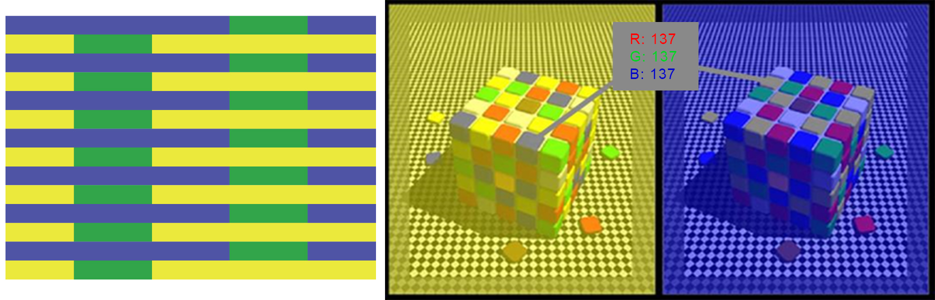
Color Temperature
Color temperature is a way to describe the light appearance provided by a light bulb (lamp) or ambient light (e.g. sky and sun) in degrees Kelvin. Typical daylight ranges from 5000 to 6500 degrees Kelvin. We use the labels D50 and D65 to indicate daylight-viewing conditions at these temperature points. Typically, commercial and residential lighting application Kelvin temperatures fall somewhere on a scale from 2000K to 6500K. A light bulb’s (lamp’s) color temperature lets us know what the look and feel of the light produced will be. The color temperature of a light bulb is assigned using the basis of correlated color temperature (CCT): Normally, temperature as a measure of the hue of emitted light only makes sense for heated metals, which glow in a certain way when heated. Depending on the Kelvin temperature that the metal object is being heated at, the glow will be various colors, such as orange, yellow or blue. The color temperature of light bulbs (lamps) is meant to replicate the Kelvin temperature of the metal object. A similar simulated temperature is used for measuring the appearance of natural lighting. Since the appearance of a luminaire represents the maximum lighting contributing to an environment (all subsequent reflection of light attenuates the initial power contributed by the light source), the temperature of the maximum color is the white point of the lighting produced, i.e. the appearance of "white" in the illuminated environment.
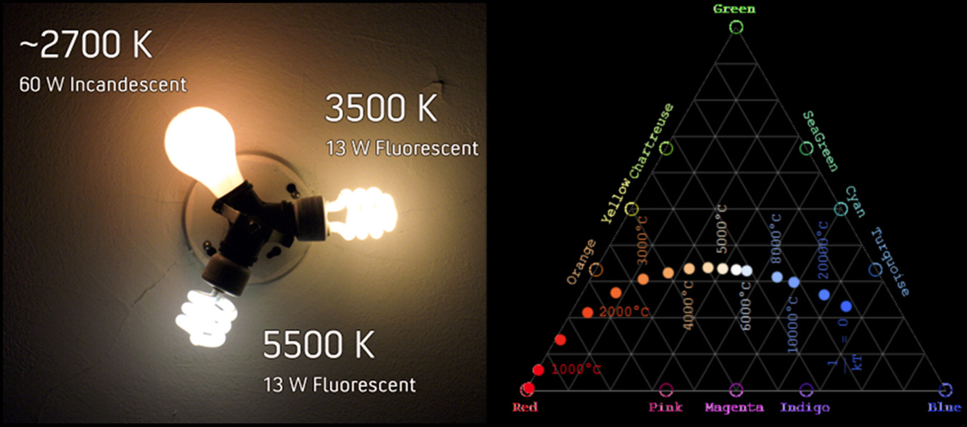
Remark: Why is temperature important in color management, reproduction and digitization? Because in order to record, recover and represent the reflectivity of artefacts being digitized and subsequently displayed, as accurately as possible, we must compensate for the color shift due to the artificial or natural lighting that is being used.
Additive and Subtractive Primaries
We refer to the red, green, and blue color set (RGB) as the additive primaries. When we combine or add all three of these, we get the entire spectrum and, thus, white light. This is the primary color set involved whenever we talk about the transmission of light, such as the display on a computer monitor, a tablet, or from a projector. For this reason, red, green, and blue are also referred to as the transmissive primaries. Here we are adding light to light, as we are overlaying luminous energy, so the production of a brighter color is to be expected. The combination of red and green light produces yellow, combining green and blue gives us cyan, while the combination of red and blue produces magenta.
Since each one of cyan, magentda and yellow is produced by subtracting one of the additive primaries from the full complement of white light, we refer to this color set (CMY) as the subtractive primaries. Each of the subtractive primaries acts as a filter for its complementary color in the additive primary color set. Cyan absorbs all red light, reflecting only green and blue. Magenta absorbs all green light, returning only red and blue; while yellow absorbs all blue light and reflects back only red and green. Just as we can produce any color sensation in the transmission of light by mixing the appropriate quantities of red, green, and blue, we can produce the corresponding color sensation when we put ink on paper by absorbing the necessary portions of the visible spectrum so that only the required amounts of red, green, and blue are reflected back. This is how cyan, magenta, and yellow work as our primary colors in the printing environment, and why we also call them the reflective primaries.
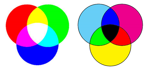
Monochromatic Images
Images captured from real-world objects record the light reaching a sensor after being scattered on or through a medium and therefore modulated by its intrinsic material properties. Additionally, the viewing angle and light direction significantly affect the light-object interplay and produce a different outgoing radiance towards the sensor. If we remove the color characteristics of light, we are left with achromatic light, which is solely characterized by its luminance. When captured as an electrical signal, this excitation is converted to some subjective brightness value that is typically scaled to a range according to some minimum and maximum values. We frequently logically map this range to normalized intensity, with the values represented by a real number between 0 (black) and 1 (white); values between these two extremes define different shades of grey, i.e. we have a grey-scale image. Finally, these grey-scale values are typically scaled to the maximum value represented by an integer format and quantized. For example, a grey-scale image with values in the normalized range is stored as an 8bit image by the conversion .
Dithering
In certain situations, where we have abundant spatial resolution and can trade it for grey-scale resolution, we can effectively mask deficiencies of the color representation quantization levels by superimposing a noise-like pattern to the image, a processed called dithering, thus suppressing banding artifacts. The human eye is quite bad at discerning high-frequency patterns and locally varying the contrast can effectively take advantage of its perceptual deficiencies to create the illusion of better brightness grading.
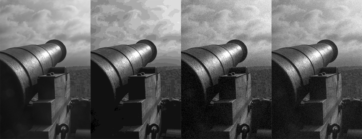
Gamma Correction
Photography and computer-generated images capture light in linear luminance space, i.e. as received by the "sensor". However, as already mentioned, we perceive these values non-linearly. If we convert the linear range to a fixed-quantization representation (e.g. RGB color with 8 bits per color channel - 24bit color images), we discriminate dim color transitions (images appear quantized) as we boost low luminance value differences. Furthermore, we fail to differentiate bright differences, thus wasting bits in our numerical representation.
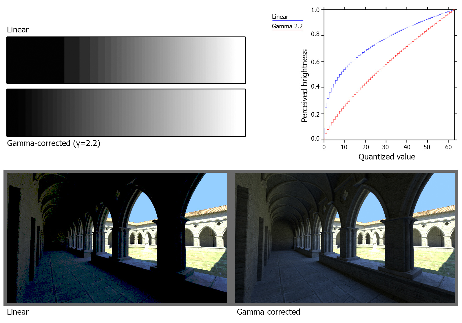
In order to allocate more bits where they count, we perform a non-linear mapping of the linear luminance scale of the raw input before encoding and storing the image data. Then in order to properly display the information, we apply the inverse intensity transformation to the data prior to sending them to the output (display or printed media). This process is called gamma correction and is implemented via two simple transformations, gamma compression and gamma expansion:
In the above equations, (called an encoding gamma).
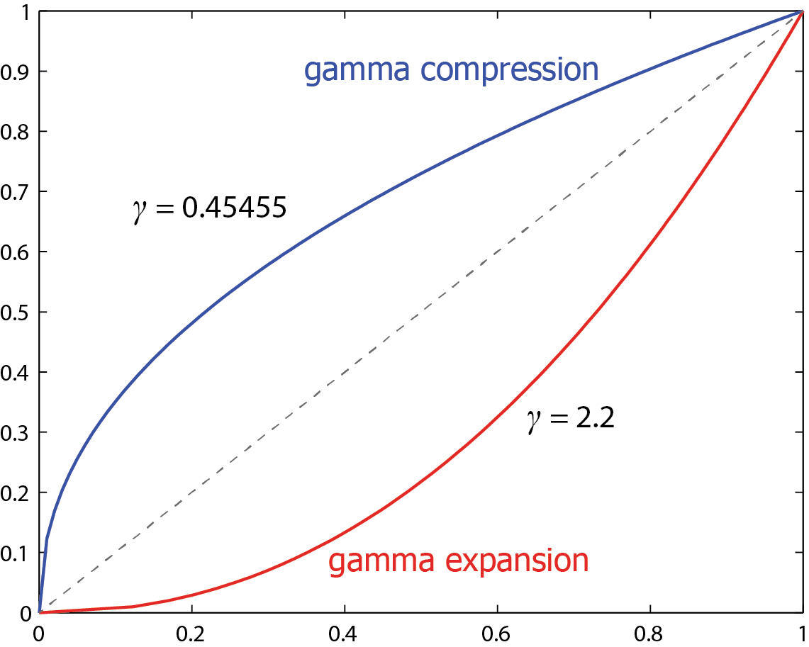
Color Models
In a world so rich in colors, there are actually no colors. Our perception of color stems from the reaction of our brain to the wavelengths of light that enter our eyes. Given the overwhelming number of different colors that can be observed in nature, we have had a long-standing desire to communicate and use color in a consistent manner. We have thus been striving to invent models for systematically describing, comparing, classifying, and ordering colors; such a model is referred to as a color model. Naturally the simplest approach was tried first, the linear model of Aristotle. Aristotle was inspired from the cyclical succession of colors that form the continuum of day and night. Unfortunately, this simple color model is a long way from reality. Plato and Pythagoras invented more elaborate color models and some of their ideas persisted until the Renaissance.
An important classification of modern color models is based on whether they are device-independent. In a device-independent color model the coordinates of a color will represent a unique color value, according to human perception. In contrast, in a device-dependent color model the same color coordinates will produce a slightly different visible color value on different display devices. The Commission Internationale d’Eclairage (CIE) has worked on producing device-independent color models; such models are useful, among other things, for the consistent conversion between device-dependent color models. For example, the red-green-blue (RGB) and cyan-magenta-yellow (CMY) models are device-dependent while CIE XYZ is device-independent.
Some device-dependent color models also follow the respective devices’ philosophy of producing arbitrary color from primary colors; we can distinguish between additive and subtractive color models. Additive-scheme color spaces can be called tristimulus color spaces, since they work by defining the amounts of three stimuli provided to the eye (the three primaries). Another important characteristic of color models is perceptual linearity. If the perceived difference between two colors is proportional to the difference of their color values across the entire color model, then the color model is perceptually linear and offers the same perceptual color precision throughout its range. Finally, it is desirable that a color model is intuitive in its use.
In the sequel, a small selection of color models are presented, based on their relevance to imaging and visualization. There exist a large number of additional color models (Wyszecki and Stiles 2000), including models that were developed for television (such as YUV, YIQ, YCbCr and YPbPr) and proprietary models (such as Kodak’s YCC).
A color space maps a range of physically produced colors (from mixed light, pigments, etc.) to an objective description of color sensations registered in the eye.
Color Gamut
Mathematically a color space is a continuous and potentially infinite domain, where color vectors can be defined with arbitrary values. For example, if we consider the (device-dependent) RGB color space, where individual components (or channels) express the emissive power of the corresponding wavelength, in theory the colors produced for each one of the R,G and B channels is a continuous infinite positive value. However, devices have physical limitations and the range of reproducible values is only a bounded subspace of the mathematical color space. This particular effective domain is called a color gamut.
The LMS Space
As noted in the introduction, our photoreceptors are tuned to specific wavelengths of light. These three wavelength regions are named as L, M and S, after the terms "long", "medium" and "short" (wavelengths) that correspond to the approximately red, green and blue stimuli related to our cones. We can think of the stimulus triggering a signal to each one of the L, M, S cones as a "coordinate" of a color space. The problem with this intuition is that our receptors are not singularly tuned to a specific wavelength but rather a whole range of them. Therefore, it would be impossible to represent a color corresponding to any specific wavelength with one component and a zero contribution of the other components, since the stimuli are always mixed together due to the overlap of their ranges. In fact, in order to represent individual wavelengths, "negative" values for each one of the RGB stimuli must also be used. This renders the basic additive stimuli modelling an unintuitive color space for representing colors and has lead to the advent of the XYZ color space.
The XYZ Color Space
In color science, Grassman’s first law states that any color can be created as a linear combination of three basic colors, provided that no combination of any subset of the basic colors can produce another. This is analogous to the linear independence requirement for the basis vectors in a coordinate system.
Aiming to provide a standard way to describe all colors, the CIE defined the XYZ color model in 1931. This is now considered as the mother of all color models. Colors are represented in a three-dimensional color space whose axes are defined by the basic colors , and ; mixing the basic colors in suitable proportions and produces all visible colors. , and are actually not visible colors themselves but must be simply regarded as computational quantities. In fact and provide chromaticity information (what the color is) while corresponds to brightness or the luminocity.
When judging the relative luminance of different colors in well-lit situations, humans tend to perceive light within the green parts of the spectrum as brighter than red or blue light of equal power 2. The luminosity function that describes the perceived brightnesses of different wavelengths is thus roughly analogous to the spectral sensitivity of M cones. The CIE model capitalises on this fact by defining Y as luminance. Z is quasi-equal to blue stimulation, or the S cone response, and X is a mix (a linear combination) of cone response curves chosen to be non-negative, in order to be able to represent "generated" colors by real sources. The XYZ tristimulus values are thus analogous to, but different from, the LMS cone responses of the human eye. Defining Y as luminance has the useful result that for any given Y value, the XZ plane will contain all possible chromaticities at that luminance.
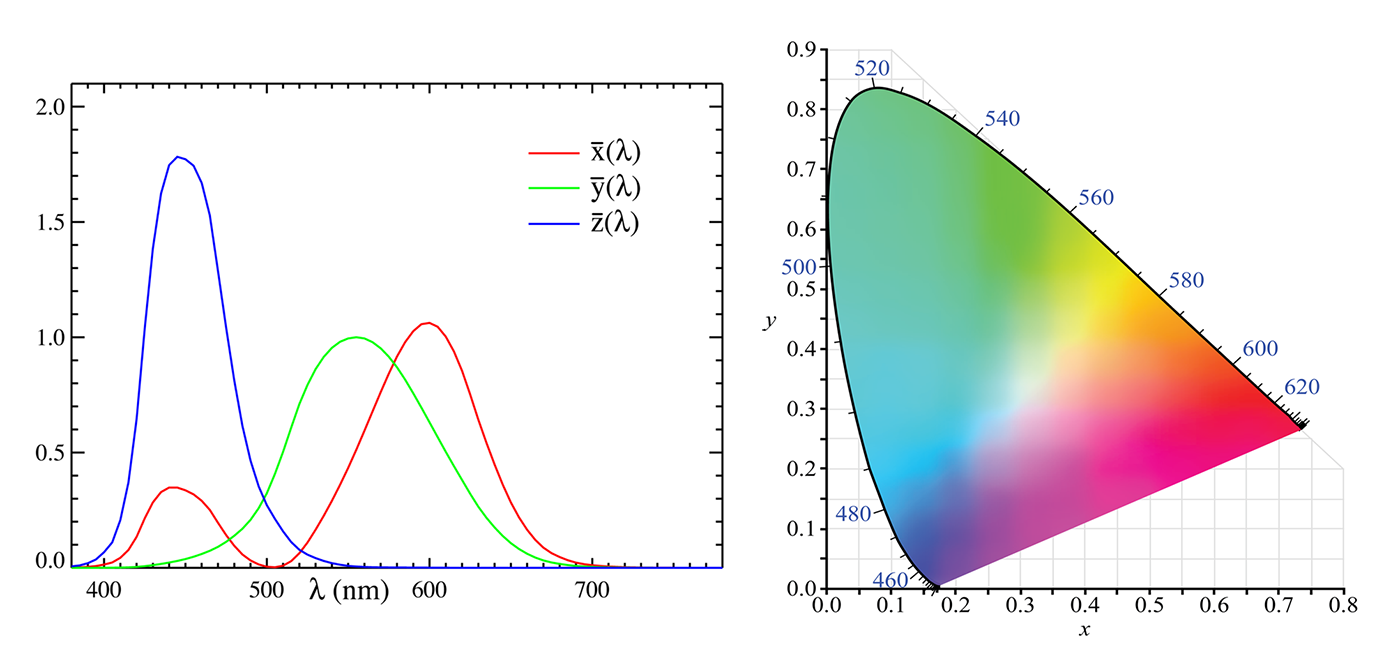
Is there a "true" white? White is associated with the maximum "value" (that being emission or reflectance) under specific conditions. So, to answer the question, there is no single chromaticity that corresponds to a "true" white. The white point is defined as the chromaticity of the color indicated when an illuminant produces an output with maximal (equal) additive values.
There are a number of standard illuminants, with specified chromaticities (in fact, specified spectra) that can be thought of as “specific kinds of white”, as discussed in the section above about temperature. Since the XYZ model is trying to be an objective one, the XYZ white point is defined as the chromaticity at which all wavelengths contribute equal power to the generated light, in other words, the light has a flat spectrum. The closest real conditions that match the flat spectrum response is the D55 standard illuminant, which is representative of “mid-morning/mid-afternoon daylight”.
The CIE XYZ color space is the most common way in technical colorimetric work to describe the color of light. For example, in the specifications for other additive color spaces (such as sRGB), the chromaticities of the standard primaries are defined in terms of their coordinates. When equations are given to allow the description of a color to be transformed from expression under one color space into expression under a different color space, most commonly the transform is given in two steps, first a transform from the “source” color space to the CIE XYZ color space, and then a transform from the CIE XYZ color space to the “destination” color space.
The RGB Color Space
As its name implies, the basic colors in the RGB additive color model are Red, Green and Blue. These basic colors were chosen, due to the correspondence with the L, M and S photoreceptors of our own vision system. On most computer displays, colors are created using an additive method. Additive color mixing begins with black ( - no light present) and ends with white (the sum of all basic colors at maximum emissive intensity - ). As more color is added, the result is lighter and tends to white. However, the notion of "maximum brightness" or "maximum reflectance" only makes sense for emissive devices and reflective surfaces, respectively. In general, luminous energy is unbounded and should be thus represented in a graphics system in order for the radiometric or photometric data to be properly represented and stored.
Color mixing and interpolation can be defined in a manner similar to the XYZ model. Within the space of the RGB cube, colors correspond to vectors from the origin , which is the black point. For a bounded RGB space, white is then , green is , etc. In this representation, the direction of a color vector defines chromaticity and its length is the intensity. The main diagonal of the RGB cube consists of shades of gray only (from black to white). If we disregard intensity, it is possible to represent the RGB system with a triangle which is the intersection of the RGB cube with the plane defined by the points Red , Green and Blue . All RGB colors are mapped onto this triangle, since all RGB vectors intersect it. The only information lost is intensity. Using the RGB triangle it is possible to refine the notion of chromaticity, by splitting it into hue and saturation. Hue is the dominant wavelength which gives a color its identity and saturation is the amount of white that is present in it. All hues are found on the perimeter of the RGB triangle; saturation is maximum at the center of the triangle and minimum at its perimeter. Colors of the same hue, but varying saturation, can be found on a line segment that connects a point on the perimeter with the triangle center.
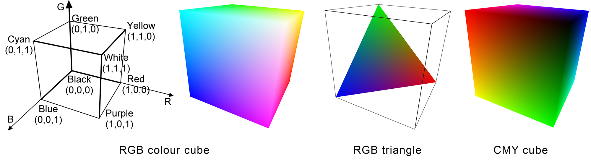
Note that due to the emissive characteristics of the illuminant, the apparent color produced may appear at different color temperature, depending on the display device. The RGB "white" only states that the maximum possible illumination level for all three components must be used. Additionally, the RGB model is not perceptually linear and, in terms of use, rather un-intuitive since it is not easy to come up with the mix of the three primaries required to produce an arbitrary color. Due to its device-dependent nature, the same RGB color triplet will potentially produce perceptually different colors on different display devices. To ensure perceptual color equality when transferring color images across RGB display devices, it is necessary to convert from one to the other via an intermediate device-independent color model.
The sRGB Color Space
sRGB is a standard RGB color space created cooperatively by HP and Microsoft in 1996 for use on monitors, printers and the Internet. The sRGB color space has been endorsed by the W3C, Exif, Intel, Pantone, Corel, and many other industry players. It is used in proprietary and open graphics file formats, such as SVG 3.
The sRGB color space is well specified and is designed to match typical home and office viewing conditions, rather than the darker environment typically used for commercial color matching. Much software is now designed with the assumption that an 8-bit-per-channel image placed unchanged onto an 8-bit-per-channel display will appear much as the sRGB specification recommends. LCDs, digital cameras, printers, and scanners all follow the sRGB standard. For this reason, one can generally assume, in the absence of embedded profiles or any other information, that any 8-bit-per-channel image file or any 8-bit-per-channel image API or device interface can be treated as being in the sRGB color space. However, when the correct display of an RGB color space is needed, color management usually must be employed.
Unlike most other RGB color spaces, the sRGB gamma cannot be expressed as a single numerical value. The overall gamma is approximately 2.2, consisting of a linear (gamma 1.0) section near black, and a non-linear section elsewhere involving a 2.4 exponent and a gamma (slope of log output versus log input) changing from 1.0 through about 2.3 (see figure next).
sRGB is sometimes avoided by high-end print publishing professionals because its color gamut is not big enough, especially in the blue-green colors, to include all the colors that can be reproduced in CMYK printing.

The CMY(K) Color Space
When colors are mixed during the painting or printing process, the subtractive color method is used. Subtractive color mixing starts with white (the color of the canvas or paper) and ends with black; as one adds color, the result gets darker and tends to black. For example, if we drop cyan paint on a piece of paper, then it absorbs the red component of incident light; if the paper is illuminated with white light then the reflected (visible) light from the painted area will be .
The CMY model is defined as the complement of RGB. Its three basic colors are Cyan, Magenta and Yellow. White appears at and black at the opposite vertex ; other colors are also in opposite vertices with respect to the RGB cube.
Being a complement of RGB, it is perceptually non-linear and rather non-intuitive, since it is not straightforward to specify a certain color as a mixture of and . The conversion from RGB to CMY is simply:
Some printing devices include Black ink in addition to Cyan, Magenta and Yellow in order to avoid synthesizing black, which appears often in text and some diagrams; they thus economize on the use of ink and provide better-quality black.
Caution should be exercised when converting from the RGB space of a display device to the CMY space of a printing device, since they are both device dependent models. The above simple transforms are unlikely to result in accurate color reproduction. Ideally, one should convert from RGB to a device-independent system, such as CIE XYZ, and then to CMY using the color profiles of the output devices.
The HSV Color Space
The amounts of Red, Green and Blue present in a color indirectly control its Hue, Saturation and Intensity characteristics. It is often simpler for humans to specify a color based on such characteristics, rather than proportions of Red, Green and Blue. One of the first modern attempts to systematically organize a color model was made by artist A.H. Munsell (Munsell and Farnum 1941). Munsell sought a conceptually simple way to universally describe color and proposed the Hue-Value-Chroma system, known today as the Hue-Saturation-Value (HSV) system, which geometrically represents colors on a cone 4.
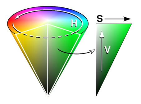
Munsell started by arranging colors on a circle, like a color wheel, encapsulating the hue characteristic. Hue is described by an angle with respect to an initial position on the circle. For example, red is found at , green at , blue at . This hue circle corresponds to a cross-section of the cone. Saturation is maximum on the surface of the cone (minus the base) which represents pure colors with maximum ‘colorfulness’; the axis of the cone represents minimum saturation (shades of gray). The value component corresponds to intensity; the minimum value indicates the absence of light (black) while the maximum value indicates that the color has its peak intensity. This component is represented by a position along the axis of the cone; corresponds to the cone’s apex and the maximum value corresponds to the center of the cone’s base.
A relatively simple linear transformation converts RGB values to HSV and vice-versa; HSV can be used in place of a device’s RGB model as a more intuitive color interface. HSV color pickers are very common in image manipulation and vector drawing tools.
Luminance - Chrominance Color Spaces
The color models in this category separate the luminance (intensity) from the chromatic value of the color. The chromatic plane is defined by two axes, each one representing opponent colors and all possible shades of the same intensity are defined on it. In the literature, chroma and luma are associated with colors that have not yet undergone a conversion to a perceptually-based scale, i.e. usually before gamma correction. Conversely, chrominance and luminance refer to colors in a perceptually corrected space, meaning that light intensity is non-linearly encoded based on gamma corrected RGB primaries.
The Lab Color Space
Once the opponent nature of color interpretation was understood, color scientists were able to create a model color space based on the opposing pairs. This is the Lab color space (Figure 3.5). The Lab variation of interest to us is officially called CIELAB. Each of the opposing pairs provides one axis of this three-dimensional color space. L is the axis for darkness to lightness; a is the axis for greenness to redness; and b is the axis for blueness to yellowness. By providing a value for each of the L, a, and b attributes, a color is accurately and uniquely located in the color space. The tremendous utility of the Lab color space is that it allows for the mathematical description of a color in a non-ambiguous and meaningful way.
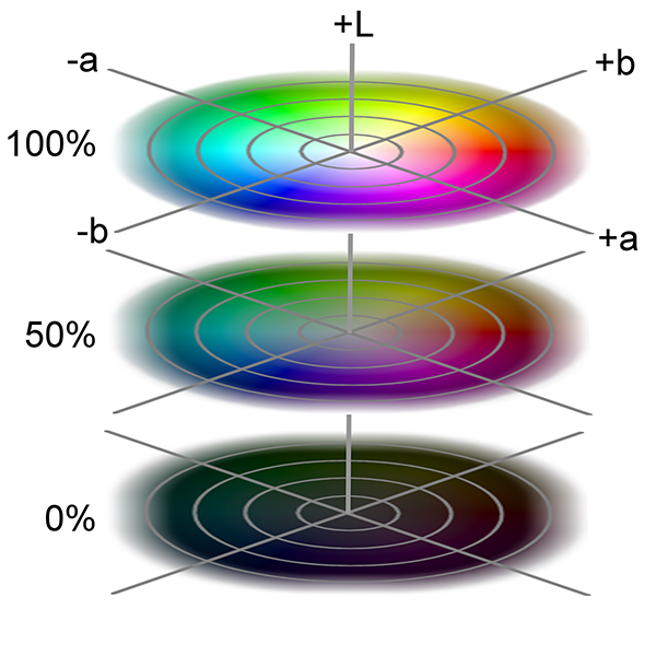
The YCbCr and YCgCo Color Spaces
and are families of color spaces used as a part of the color image pipeline in video and digital photography systems. is the luma component and and are the blue-difference and red-difference chroma components. is distinguished from , which is luminance. Typically, transformations are provided for the conversion to and from the RGB color space, since the primary use of the model is in photography and video encoding. The YCbCr model is used in the representation and compression of color channels in the JPEG image format and the MPEG-2 video format.
The YCgCo (often written YCoCg) color space is similar in nature to the YCbCr, but encodes chrominance in two different axes, the chrominance orange (Co) and the chrominance green (Cg). It is primarily used in the H.264 video format and is considered superior in terms of information decorrelation across the color planes.
An example image encoded in the two YCC formats is shown in the following figure.
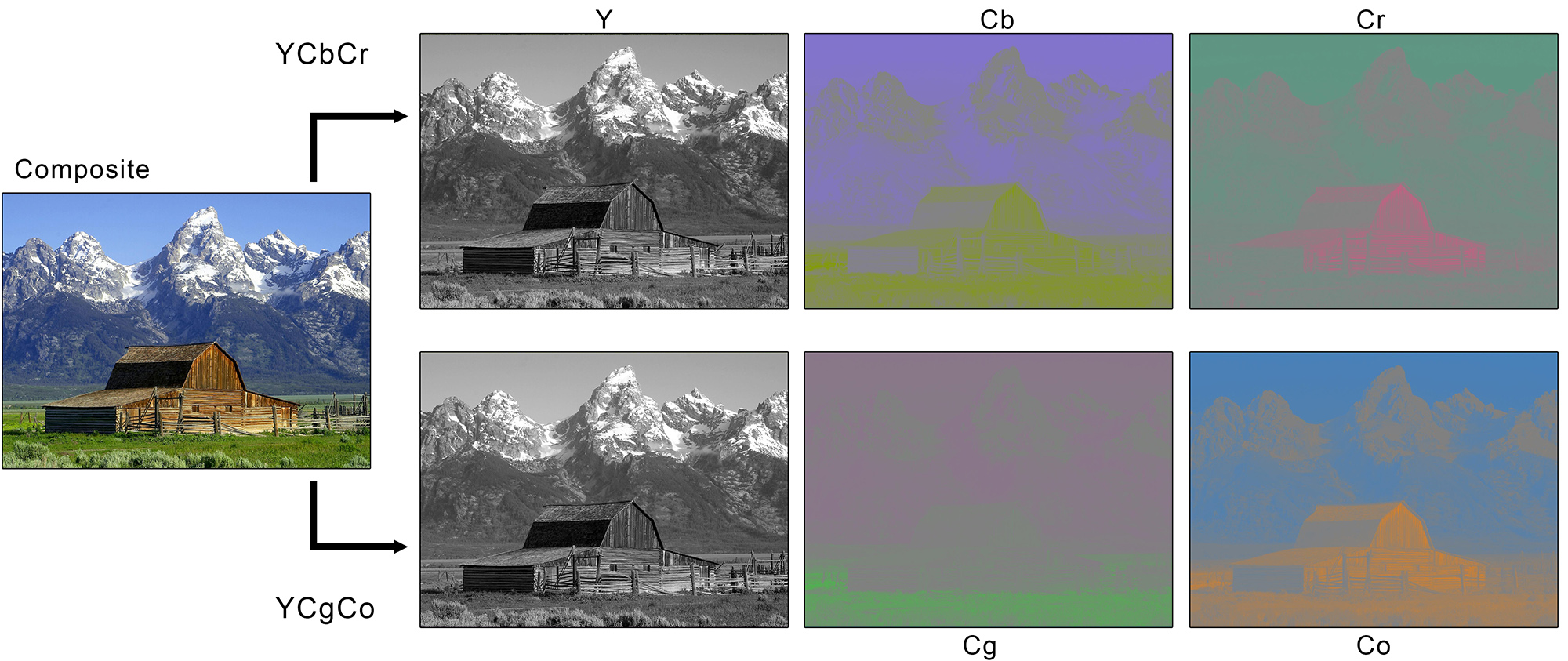
Luma - Chroma Spaces and Image Compression
The primary use of a YCC space is image compression. It allows the efficient compression of image information in a perceptually optimal manner, by retaining as much information possible in the luma channel and aggressively reducing the (spatial) resolution of the two chroma channels, as shown in the next figure. The Human Visual System luminance visual acuity is greater than the discrimination of chrominance variations and therefore we can subsample the chroma channels without much perceptual degradation. For the majority of typical image presentation scenarios, luminance is perceptually more important and with a faster variance across the image domain. However, in extreme cases, since color information is subsampled and then expanded to fill the same pixel area, sharp chromatic transitions (e.g. a red rose over a green background) will cause color bleeding and desaturation in the rectified image.