Materials and Shading Models

Materials and Appearance

The appearance of a surface or fuzzy volume is determined by the interaction of light with the medium and its transitions. Therefore, to properly set up algorithms and mathematical models to compute the lighting on the (virtual) surfaces and inside the modeled volume of objects, we must first understand how light interacts with the real, physical world.

In computer graphics terms, an object is characterized by its material, which encompasses both the substance the object is made of and the finish of the surface. The qualities that represent both aspects of the object are not necessarily uniform over the entire surface or volume of the object and we can modify and control them using the process of texturing, which we will examine next. Materials may also change over time, as their qualities are subject to physical and chemical processes or inherently volatile and/or in motion.

Light propagation in computer graphics is almost without exception modeled using geometric optics; light is considered to travel in straight path segments that connect scattering events in space. As such, we treat light incident on a surface point as coming from one or more specific directions. Similarly, we can consider rays of light emanating from a specific location and traversing space in a straight line. Geometric optics do not account for certain optical effects such as diffraction and interference, which may become relevant in situations where the micro-structure of the modeled surfaces is of comparable scale to the wavelength of the incident light.

Reflection and Transmission

Most of the light-object interaction visible to us occurs at the interface between two media. A surface interface is formed when the density of two media abruptly changes and so does the index of refraction (or refractive index). In optics, the refractive index (or refraction index) of an optical medium is the ratio of the apparent speed of light in the air or vacuum to the speed in the medium. The refractive index determines how much the path of light is bent, or refracted, when entering a material.

Since we simulate a world as observed through our "eyes", most often light is observed to interact with the surface boundary of dense media, coming from other surfaces present in the vacuum, air or water (for underwater environments). But we also often visualize the interaction of light exiting such surfaces, transmitted through the volume of objects.

On a locally smooth surface, reflected light will bounce off the surface in a direction symmetrical to the angle of incidence with respect to the normal vector of the surface, as illustrated in the above figure. Light transmitted through the surface interface will be deflected off its straight path due to refraction, according to Snell’s law of refraction, which states that $n_1 \sin(\theta_1) = n_2 \sin(\theta_2)$, where $\theta_1$ and $\theta_2$ are the angles between the light’s path and the direction perpendicular to the surface for the two media with indices of refraction $n_1$ and $n_2$, respectively. Denser media have a higher index of refraction and vice versa.

Light will keep traversing both sides of the interface after the energy split and become absorbed or scattered though particulate media or through other interfaces. The exact ratio of the energy bouncing off the surface versus the amount entering the medium of incidence is described by specific and well-studied equations of the electromagnetic theory, taking into account the polarization of incident light, the indices of refraction of the media at the two sides of the surface and the angle of incidence. In computer graphics, we usually simplify this interaction, phasing out polarization and approximating the fraction by faster-to-compute equations.

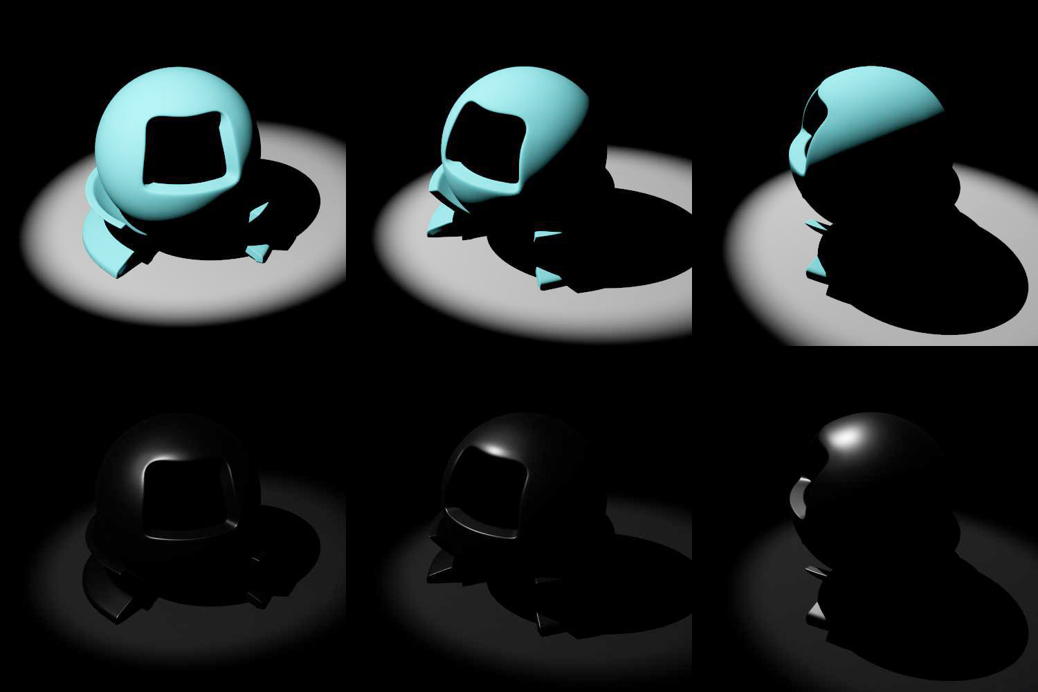
The following plots show how different materials reflect light traveling through vacuum against the angle of incidence. An angle of zero degrees corresponds to "normal incidence", i.e. the case where light strikes the medium with a direction perpendicular to the surface. 90 degrees correspond to light grazing the surface from the side.

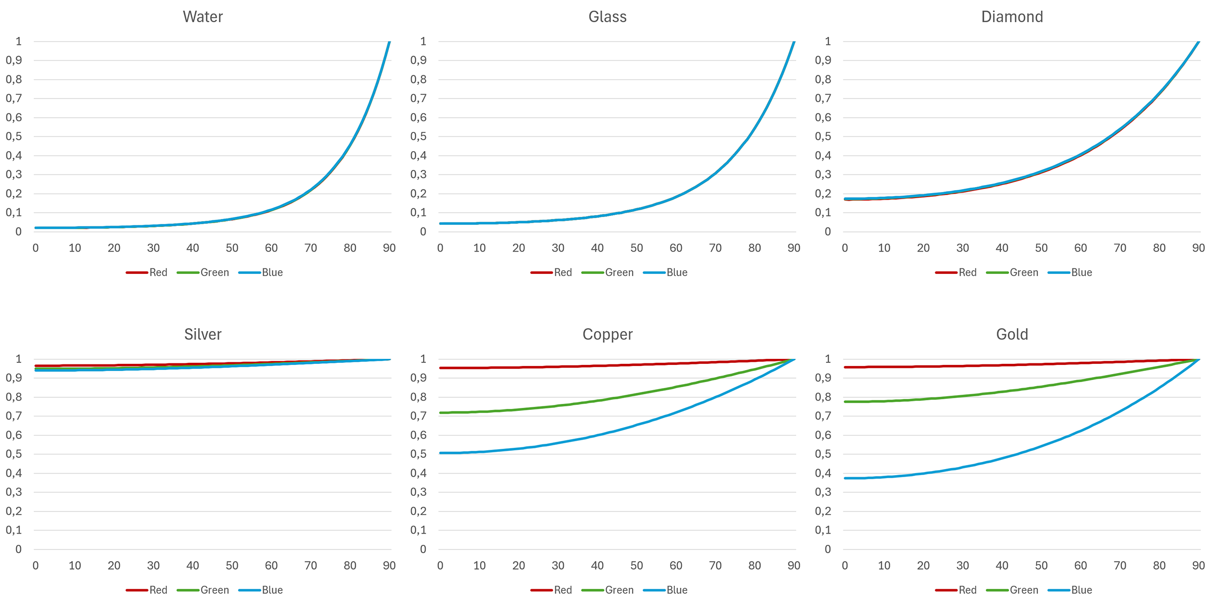
Three important observations become apparent:

• The reflectance becomes minimum at normal incidence and tends towards 100% at grazing incidence angles. This is easily observed in the example of the following photograph. This also means that conversely, transmittance is maximized at normal incidence, allowing more light to pass through the surface and scatter within the medium.

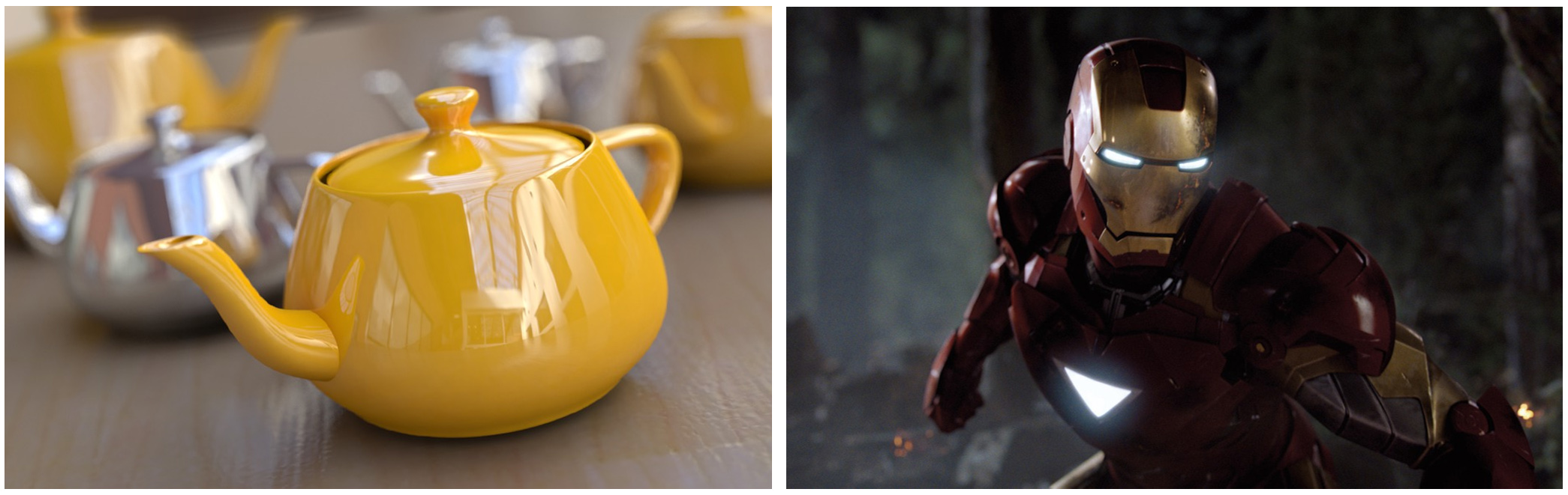
• Metals exhibit a very strong reflectance, nearly two orders of magnitude larger than insulators (non-metals). This gives them the characteristic "brightness" compared to other materials.

• The reflectance of many metals is heavily dependent on the wavelength of incident light, tinting the reflection. Two characteristic metals are gold and copper, shown in the plots above.

Scattering and Absorption

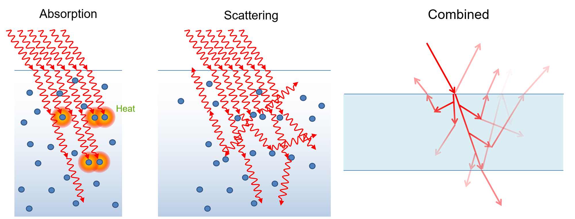
Once light passes through the surface, it starts colliding with the particles of the medium and photons are either "absorbed", with their energy being converted to some other form (typically heat), or deflected to scatter in other directions. The exact behavior depends on the type, size and density of the particles in the medium light travels through. In general, denser media have higher probability to absorb and deflect light. It is also important to note that both absorption and scattering is selective in terms of wavelength of incident light, meaning that certain colors tend to scatter or attenuate more.

Scattering is an important process for physics and computer graphics by extent. Light that gets scattered on particles inside the medium re-exits the surface of the object various locations, after bouncing off pigment particles one or more times. Since the scattering is preferential in terms of color, according to the pigments present in the matter, the light exiting the surface becomes modulated by the characteristic "color" of the material. In computer graphics, we interchangeable use the term base color and albedo to express this characteristic color (and intensity) the surface of a non-metallic object gets when white light is shone on it. It is important to understand that this coloring process is not due to reflected light, but rather due to light that is transmitted though the surface and re-emerges, after scattering back.

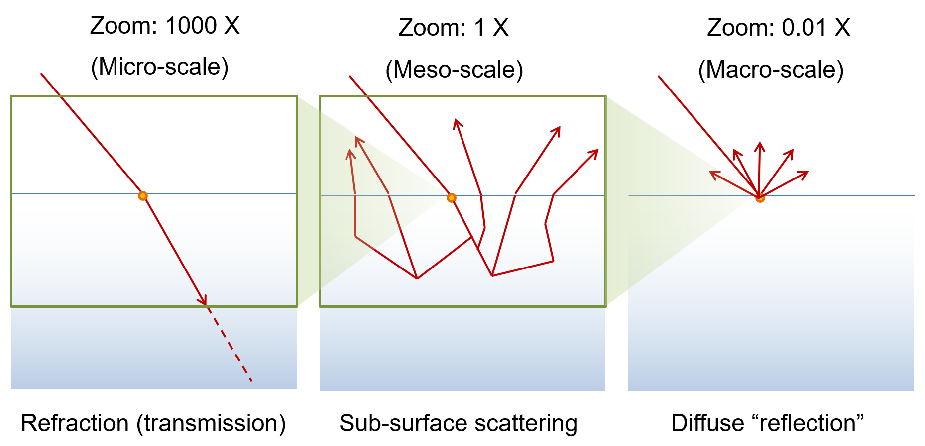
The scale at which we observe and measure the scattering of light is very important to the determination of the general appearance of objects. If we could zoom in, right at the point of incidence of light, the latter would not have traveled any distance inside the medium and on a smooth surface we would only observe the refraction of the light as it starts traversing the mass of the object in a new direction, without any out-scattering. As we zoom out, we will start registering light that gets scattered as it now moves deeper into the medium. Light will re-emerge at various points on the surface of entry or elsewhere, depending on the intensity of the scattering and the absorption of the medium. If the medium does not quickly dampen the luminous energy, it will travel long distances inside the body and we will be able to register light exiting at parts of the geometry that are significantly distant to the point of entry. We collectively call this complex interaction sub-surface scattering. However, if our scale of observation is such that the volume in which we get any noticeable outgoing lighting appears very close to the point of entry of the incident light, then the apparent effect is that of light being diffusely "reflected" on the spot. This is something very common in computer graphics, where the scale of observation is typically meso- and macroscopic, with regard to the typical absorption depth of opaque materials and surface lighting is considered in a discretized manner; you cannot sample (observe) the lighting at a finer level than the pixel unit, without averaging. For most insulators (non-metallic materials), the presence of diffusely back-scattered light is high and characterizes the material in terms of color. However, it has been often erroneously treated as reflected light, while it is not, in the physical (and mathematical) sense.

Surface Roughness

Up to now we have only considered what happens to light when striking a flat surface. But object surfaces can be rough, due to physical and chemical processes that affect the graininess and relief of their surface. This irregular morphology of a surface affects the direction light is reflected and transmitted at a statistical level, since each point of the surface may be oriented slightly differently. At a microscopic level, each "micro-facet" can be considered as locally smooth and therefore acts as an ideally flat surface. However, each facet has its own orientation and all of them are only collectively oriented "on average" according to the geometric normal of the object’s surface. This is illustrated in the following figure.

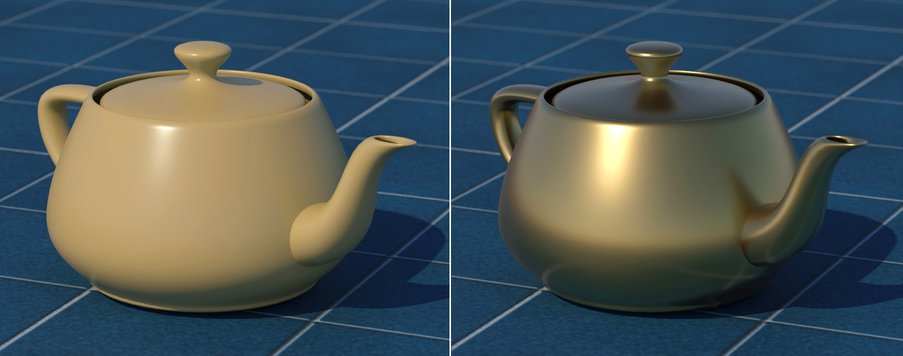
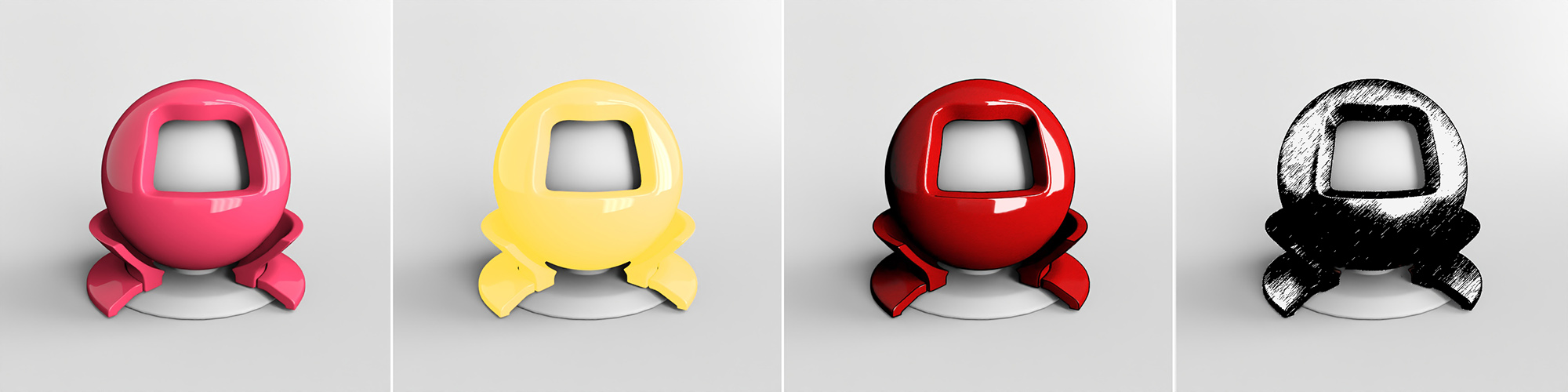
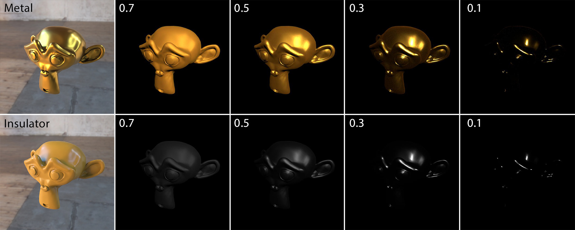
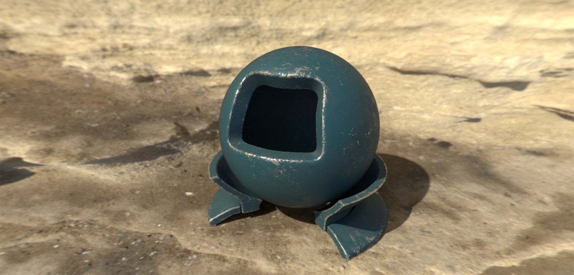
It is important to understand that the roughness (or conversely the "glossiness") of a surface is not part of the specification and description of a physical material. It is the "finish" of a surface that makes it smooth, grainy, polished in an oriented manner and so on. This means that an object made of a certain substance, can be processed to appear more or less glossy. This is shown in the following examples.

In graphics, we tend to combine the substance properties and the finish of a surface in a single set of properties that we call the "material". This in essence corresponds to the set of information that are necessary to shade a point on the surface based on its geometry and incident light.

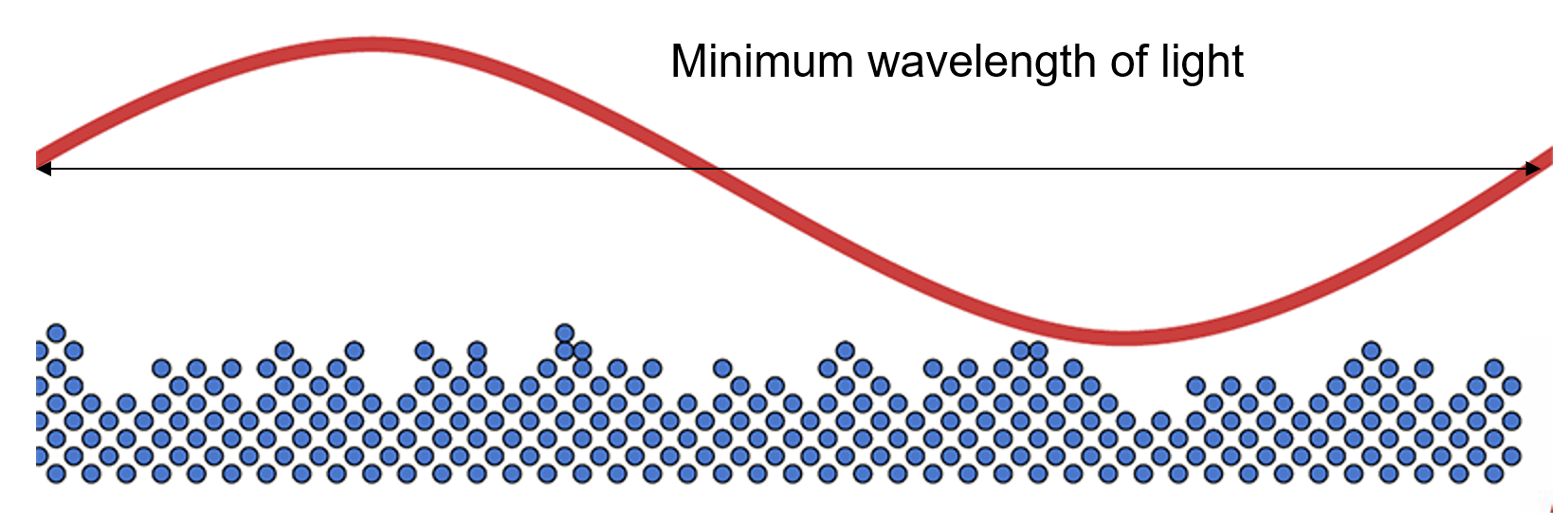
A question that is often relevant to the micro-structure of a surface is whether there is a truly perfectly smooth surface. In truth, there is no physically flat surface, as the molecular structure of an object is never ideally flat. However, the real question here is whether there is an ideal optically flat surface for geometric optics to be valid. To that question, the answer is yes, provided light is of a sufficiently low frequency with respect to the size of the surface irregularities. Typically, in graphics we can dispense with phenomena such as diffraction, which occurs when the size of surface groves is comparable to the wavelength of light and requires treating light as a wave to properly model the interaction with the surface. If required, such diffractive surfaces can be treated separately, with a specialized model. We can also consider that in an effort to polish a surface, we can attain a leveling of the surface irregularities, such that the minimum wavelength of light is far greater than the relief of the surface, lending the latter a perfectly smooth finish.

Local shading models

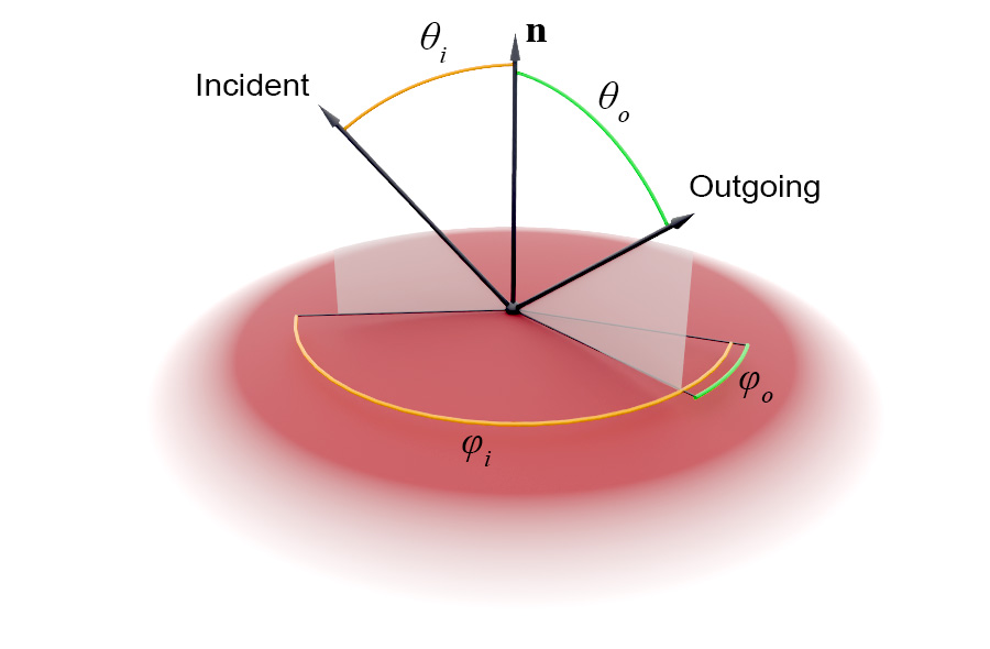
A shading model is a mathematical model that simulates the relationship between the incident light from a certain direction onto a surface point and the reflected light in another direction as well as the transmitted light through the object. We call this model a local one because it only regards the local interaction of light at the point of incidence, with no regard about the origin of the incoming light or the destination of the outgoing illumination. In other words, in a local shading model, each shaded point is treated in isolation. In computer graphics, the local shading model is represented by some bidirectional scattering distribution function (BSDF). For efficiency and clarity, we often split the equation in two parts, each handling the reflected and transmitted part of the luminous energy separately: the bidirectional reflectance distribution function (BRDF) and the bidirectional transmittance distribution function, respectively.

The term "bidirectional" refers to the fact that in many shading computations of image synthesis algorithms (see Rendering unit), we may need to follow the light as it bounces off a surface or trace its contribution the other way around, from the point of view of an observer "looking at" the given point on the surface and towards a candidate illumination direction. This means that the B(X)DF must be able reciprocal with respect to the input and output direction; it must be known when the incident and outgoing directions are exchanged. For reflection, the BRDF is the same, if the directions are exchanged, while for refraction events, due to a focusing of the resulting refraction directions, there is a corrective term to by multiplied with the BRDF dependent on the indices of refraction.

A shading model may attempt to model an as faithful to the physical world light interaction as possible, deliberately simplify computations for efficiency or even attempt to model a non-photorealistic surface response to lighting, for artistic purposes. Some examples are shown below.

Principled Shading Models

In a shading model, the energy must be properly balanced and conserved, in order for it to be physically correct, or "principled". The BSDF of the model is usually analyzed further into sub-components, each one corresponding to a specific type and stage of light scattering. Let us use the following energy distribution tree as an example of a simplified principled model to explain this.

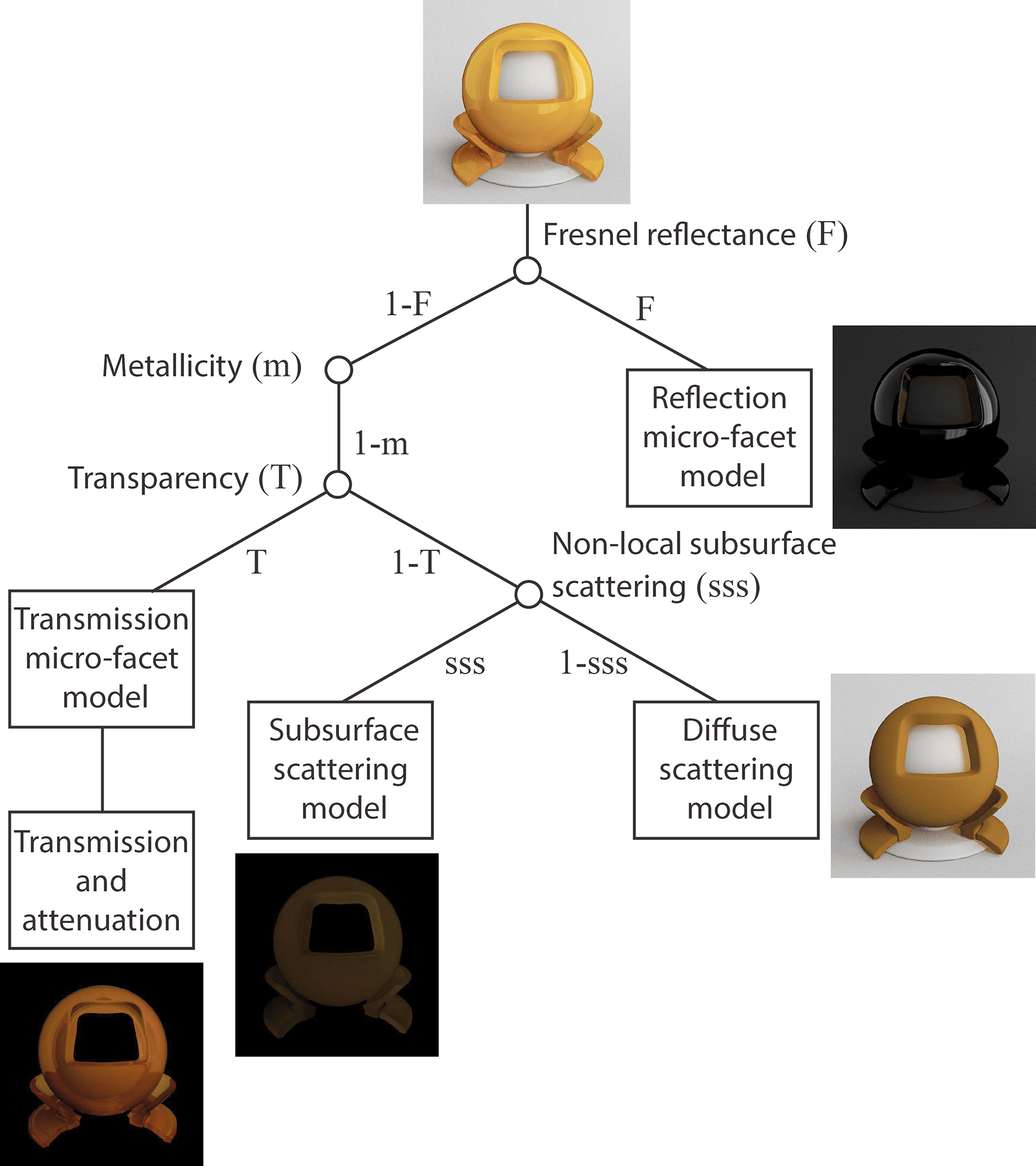
At a light-surface interaction event, we must first calculate how much light is immediately reflected back. We typically employ some approximation of the Fresnel reflectance formulas for unpolarized or polarized light to determine the Fresnel reflectance $F$ of the surface due to the particular angle of incidence. For the reflected part, the contribution of the incident light to the specific outgoing direction of observation is computed, using the normal vector at the point of incidence, the reflectance at normal incidence and the properties of the surface finish (see micro-facet models below).

The remaining portion of the energy ($1-F$) that is not reflected, enters the surface with a directional distribution dictated by the micro-facet transmission model employed. If the medium is metallic, no light propagates further¹ and the only contributing factor is the reflected light. If the medium is an insulator, 3 effects must be considered and balanced for energy conservation: immediate back-scattering, or diffuse reflection, non-local subsurface scattering and transmission through the medium on a straight path with energy attenuation. In the most simple rendering algorithms, only reflection, diffuse scattering and transmission are considered. In other rendering paradigms, such as path tracing, sub-surface scattering and transmission are combined using a series of scattering events inside the participating medium. There are also several approximation models for the fast rendering of subsurface scattering, that are not physically correct per se, but provide a plausible lighting for real-time rendering applications.

Next we examine the two most common models used for describing the scattering of light at the point of incidence.

Diffuse Scattering

The back-scattering of light immediately after entering a surface is the dominant effect for insulators that are not clear media. Plastics, ceramics, food, wood, paper, cement and other everyday materials have a characteristic color due to their raw substance or due artificial pigmentation. The most important property of that sort of scattering is the randomness of the outgoing dispersion direction that results in a very uniform distribution of the scattered light. This translates to the apparent illumination due to diffuse scattering being independent of the viewing angle (outgoing light direction), as demonstrated in the following example. Therefore, the outgoing direction is phased out of the relevant computation, greatly simplifying the diffuse illumination model. Reflected light on the other hand, no matter how rough the surface is, is dependent on the outgoing direction and cannot be simplified.

We typically express the intensity of the diffuse scattering by providing a base color or albedo for the surface.

Micro-facet Models

Rough surfaces affect both the reflected and the refracted light similarly, as they deflect light in multiple directions, according to their micro-structure. The conceptual model that is commonly used for deriving the formulas for the BRDF and BTDF of rough surfaces is the Torrance - Sparrow micro-facet model (Torrance and Sparrow 1967). In this widely adopted modeling of rough materials, a surface is assumed to be composed of long symmetric V-shaped grooves, each consisting of two planar facets tilted at equal but opposite angles to the surface normal (see figure below). In order to estimate the response of the reflective surface to a given direction, the facets are considered perfect mirrors and therefore reflect light only in the direction of perfect reflection. The elevation (slope) of the facets $\theta_{a}$ as well as the orientation of the cavities (azimuth) are determined by a statistical distribution that characterizes the surface finish.

In order for the Torrance-Sparrow model to work, the area $da$ of the micro-facets is small compared to the inspected area $dA$ near the point of light incidence. Also, the wavelength $\lambda$ of the incident light is supposed to be significantly smaller than the dimensions of the facets in order to avoid interference phenomena and be able to work with geometrical optics.

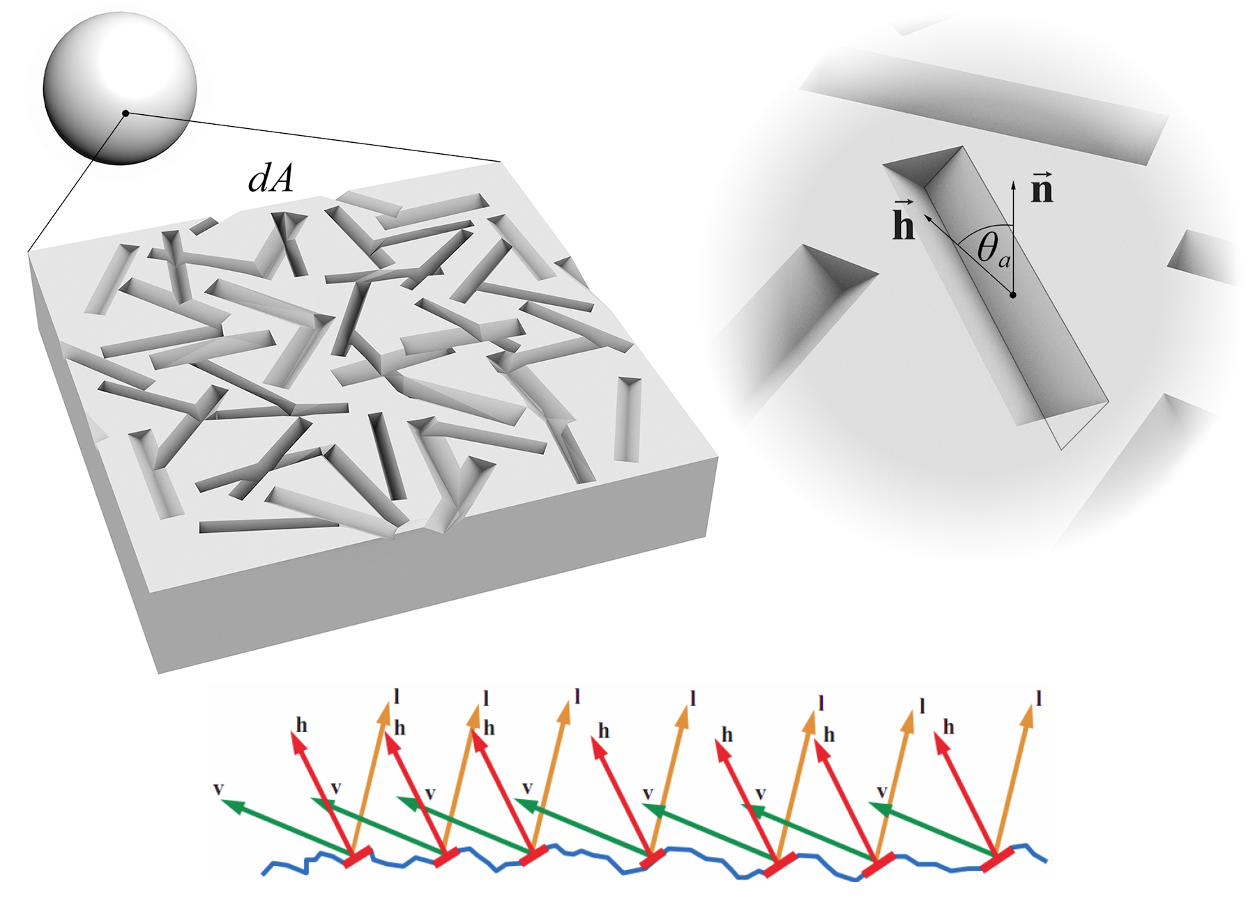
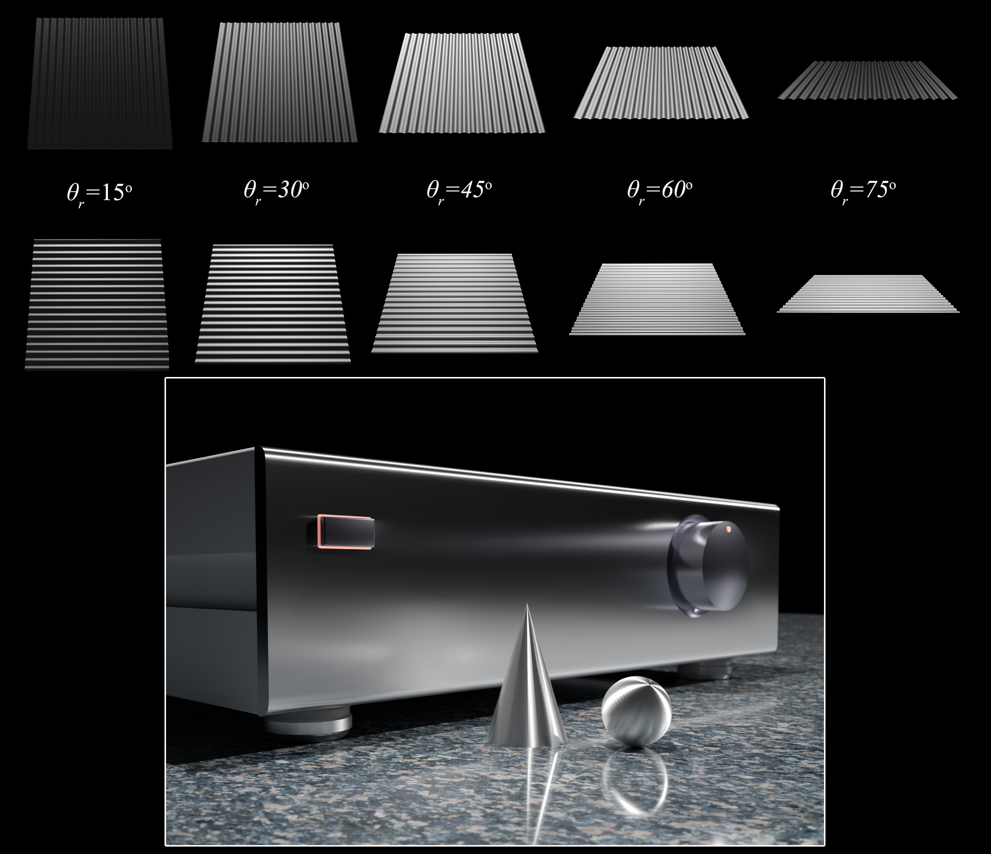
The shading models that have been developed based on the Torrance - Sparrow micro-facet model provide a reflection (and transmission, respectively) fraction of the total reflected (or refracted) energy that passes from a given incident light direction to an outgoing observation direction and vice versa. The BRDF (BTDF) is parameterized according to surface roughness, which in turn controls the statistical behavior of the micro-facets’ alignment. The primary computation inside such a model answers to the question "what is the percentage of the micro-facets that are aligned in such a way so that light is deflected from the given input direction to the given output direction" (see bottom inset in the figure above). Additional factors are considered for further dampening the response of the surface to light, such as the occlusion caused by the microscopic grooves themselves, when light strikes or leaves the surface at a low angle.

As can be observed in the above figure, increasing the roughness spreads the incident light into a wider lobe of scattering directions. Due to the requirement for energy preservation, though, a physically correct model suppresses the brightness of the reflected light so that the total energy leaving the surface in all directions remains the same, regardless of roughness.

The Importance of Scale

As mentioned in the decomposition of the various processes that are in effect in light scattering, the apparent lighting is greatly related to the scale of observation. We have already seen this in the case of sub-surface scattering, but it is evident in all aspects of material modeling for visualization. Scale affects what is considered the "local neighborhood" of the point of incidence. The assumed extent of this local neighborhood greatly affects the statistics of the shading model employed and therefore its parameters must be carefully chosen to match the scale at which the vicinity of the incident point is observed. This is best explained with an example.

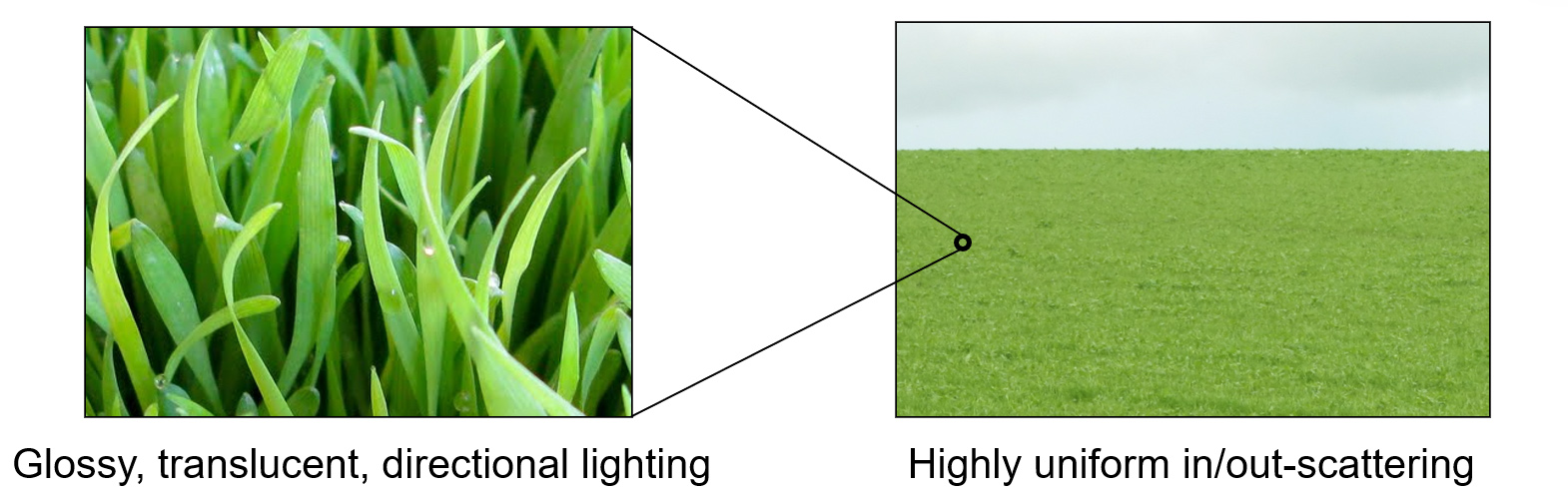
The grass blades, when observed at close distance, are in general glossy and translucent, with a directional reflection and sub-surface scattering that create view- and surface-orientation-dependent lighting. Zooming out to view an entire field of grass, the appearance is entirely different: The resulting scattered illumination is highly diffuse and uniform, like observing a cloth made of a dense woven fabric. The individual structure of the blades that we could see at high magnification was macro-scale geometry and the smooth surface and low profile of each blade was defining the observed material. When observing the field, the grass blades became micro-structure for the subtended area within each pixel and, combined with the mutual occlusion of the blades, provided a completely different statistical landscape and therefore illumination.

Texturing

Introduction

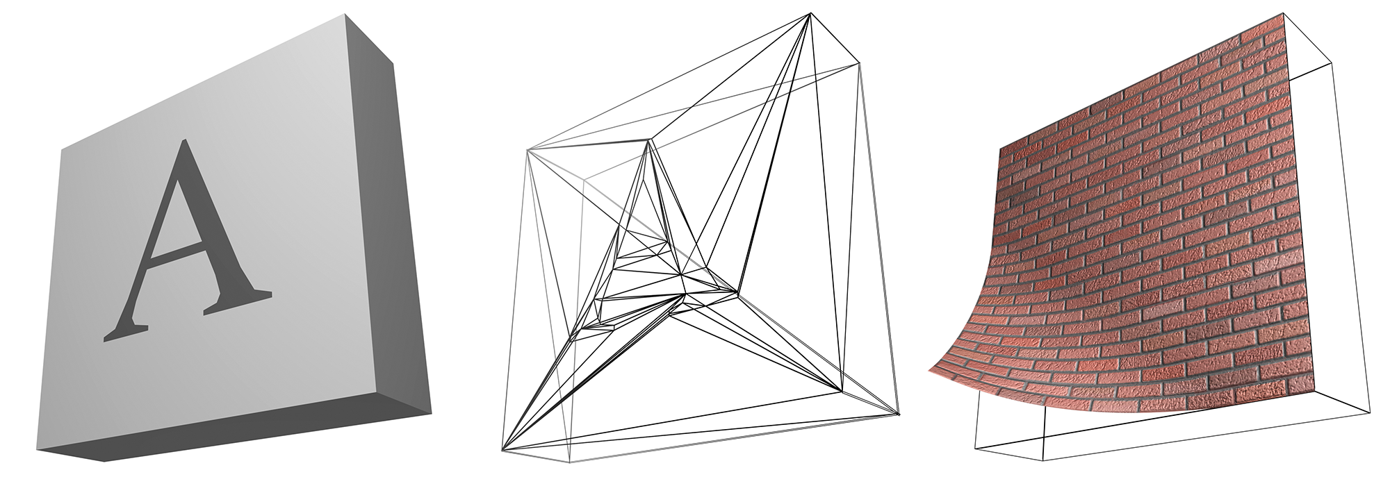
In the real world, surfaces very seldom exhibit a uniform appearance. Material properties, including albedo, Fresnel reflectance and roughness, vary across the object and the resulting appearance must be modeled in the virtual world, using computer graphics. Material properties can be assigned to vertices of polygons or entire clusters of geometric primitives and accessed via a shading algorithm to obtain the shading parameters and perform a local shading computation. Unfortunately, this primitive-dependent variation of the material properties over the surface of an object is very unlikely to occur in a real environment. In practice, on every surface, from the most dull and uninteresting real objects to the most intricate ones, one can detect small imperfections, geometric details, patterns or variations in the material consistency. These variations are perceived by the human eye and help us identify objects and materials and determine the physical qualities of the various media. It is often possible to represent the apparent discontinuities or transitions of the material properties as changes in the surface structure and vertex properties. This might even be an efficient modeling approach in the case of plain and well-defined patterns, as is the case in the first two insets of the following figure. In this particular example, a planar polygon is split at the boundaries of an A-shaped embedded pattern of a different color than the rest of the surface. But what if the desired pattern is more irregular and complex, as is the case of the material of the surface in the third inset? Clearly we need a different approach to modify the local material behavior across a polygonal or otherwise defined surface.

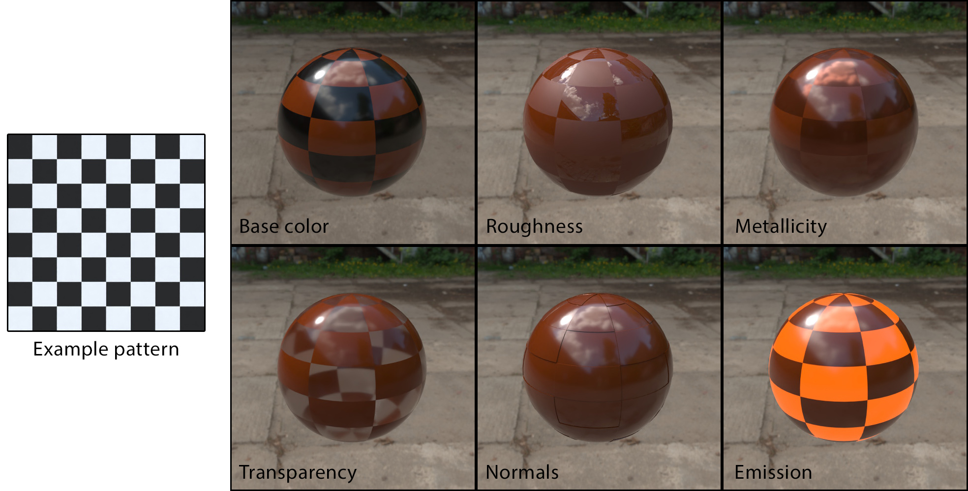
Texturing deals with the mechanism of spatially varying one or more of the material attributes of a surface in a predefined manner, without affecting the underlying topology of the geometry. These attributes can be anything from the color and the transparency of the surface to the local normal and reflectivity at a given point. The association between a given surface point (or one of its local properties, like the normal vector) and a material value in the texture space, where the desired pattern is defined, is done via a texture mapping function. The pattern itself can be a one, two or three-dimensional array of samples (a texture map) or a procedural shader. Depending on the attribute of the material that is affected by texture mapping, the result can be a scalar value, as in the case of surface roughness or alpha value, or a vector, signifying an RGB color value, a new local normal vector etc. Multiple textures can be applied to a single surface in order to modify one or more of its material properties. Different texture mapping functions may be associated with a single attribute and combined under a texture shader hierarchy.

Types of Texturing

A texture is most often defined as an array of values (an image, in the general sense) of 1 to 3 dimensions, representing some sampled content. Any texture form can be also considered to be temporally evolving (animated), adding yet another dimension to its parameterization. The content itself can be anything from captured and processed images, digitally created patterns and images, or simulated and computed data. This is probably the most flexible form of texturing, as it allows the independent specification of textural content at every location. However, image-based texturing is discretized at a specific resolution and therefore suffers from the same artifacts and limitations inherent in every sampled content. We will discuss more about these shortcomings and ways to alleviate them below, as image textures are very important to graphics, and particularly real-time rendering.

An alternative way to represent textural information is via a mathematical function or algorithm, which directly maps a 3D coordinate or parametric location on a surface to a texture value. Procedural textures are a powerful tool due to three main reasons:

• Their spatio-temporal behavior can be easily controlled globally by a small number of parameters, offering infinite variations.

• They inherently have an "infinite resolution", since they are not sampled values, but rather on-the-fly computed values.

• They can be combined using function composition to represent increasingly more complex and interesting patterns.

Procedural texturing has been extensively used in cinematic computer graphics, often combined with texture images. They are also particularly useful in the texture creation pipeline, to compose new texture images.

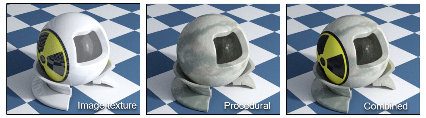
Image-based Texturing

A texture image (or simply a texture map) acts as a look-up table of discrete values and is actually typically sampled as such. Similar to any look-up table, it maps a range of a parametric space to a set of discrete samples of the texture attribute. Values in-between registered samples are estimated using some form of interpolation to "fill in the gaps" between known values. We often call the parametric domain where the texture is defined, the texture space. Its dimensionality corresponds to the number of independent texture parameters or dimensions of the texture map.

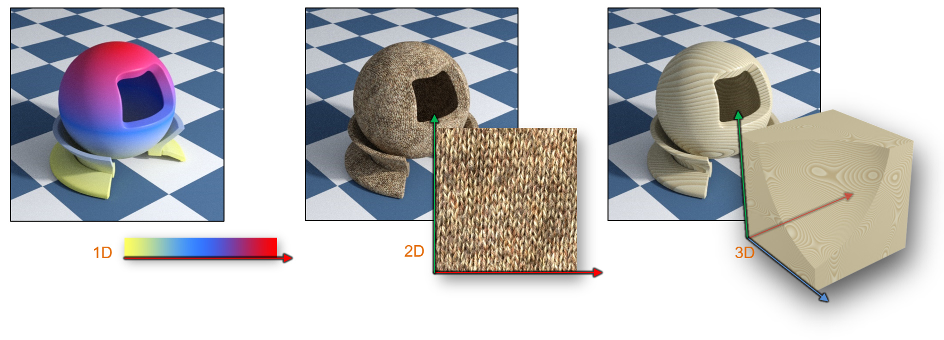
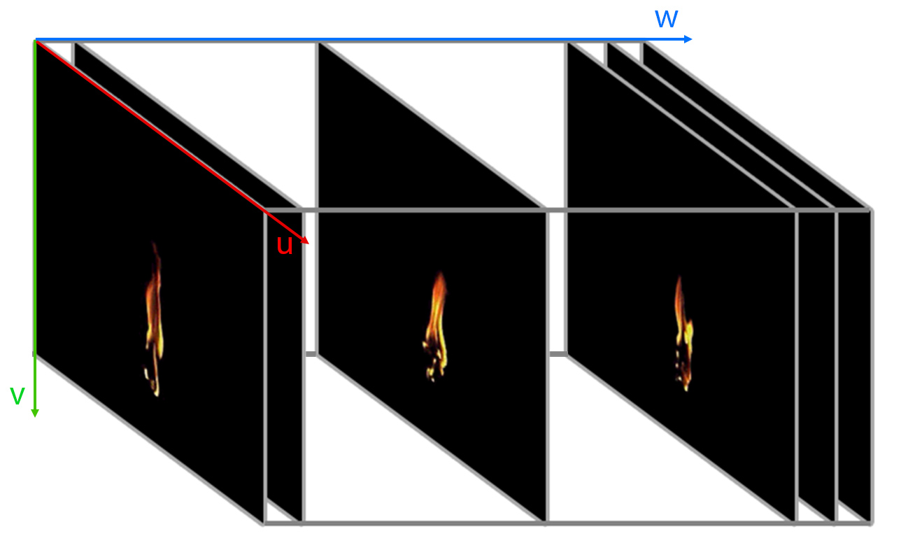
A one-dimensional texture is simply a linear collection of different values, materializing a simple look-up table indexed by a single parameter. Similarly, a two-dimensional texture is akin to a bitmap and it is typically implemented and stored as such, too. Digitized, created and processed content often ends up as a 2D texture to be used for rendering and, aside from 3D geometry, this is the most common asset used in interactive and offline rendering applications. Contrary to a 2D texture map, a 3D image texture is constructed so that it represents the variation of an attribute over the entire 3D domain, including the internal volume of objects instead of just their surface. In this sense, this is a volumetric texture. Alternatively, the three-dimensional parameterization can be split into a 1D stack of 2D textures, representing the evolution of a two-dimensional texture over time. For example, a sequence of frames from a video can be loaded into a 3D texture, each frame stored as a slice of the volume texture. We can then play back and loop through the slices of the volume, presenting an alternative 2D texture map according to the 3rd texture parameter (time).

To differentiate the notion of an elementary sample of a texture from a pixel (picture element), which is typically defined in an integer lattice that represents a bitmap, a texel is the smallest fragment of the texture space interval that corresponds to a single sample. Thus it can be one-, two- or three-dimensional in nature.

Texture Parameterization

To apply a texture map to a surface, we need to be able to define a mapping between the surface primitives and the space where the textural information exists. The parametric domain is usually considered normalized and independent of the actual resolution of the image. This is very important since a single texture map projected on a surface can be of different resolution depending on the application requirements and the rendering system capabilities. Using the pixel coordinates of a bitmap directly would be problematic, since these would be bound to a specific image resolution. By abstracting the position on the image using a normalized interval for each coordinate, we effectively decouple the indexing of the texture from the actual representation fidelity of the sampled information.

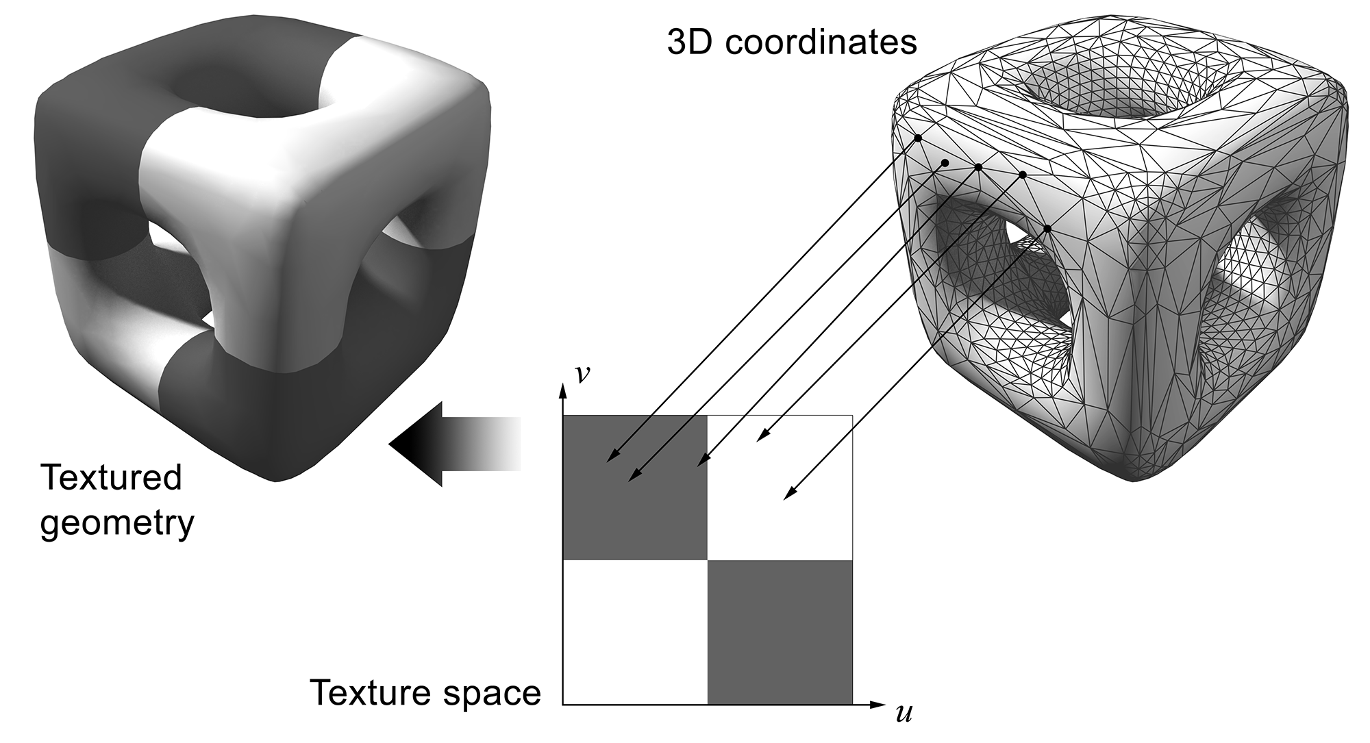
To define the correspondence between a surface point and the texture space, i.e. its texture or uv parameterization, we typically employ some form of automatic mapping function to collections of primitives, which can be later modified either algorithmically or manually, via the appropriate texturing mapping tools. There are infinite ways to map surface locations to the parametric domain but not all of them are convenient or meaningful. The uv parameterization must be defined in such a way that facilitates the laying of a textural pattern on the 3D surface, so that its features wrap over the geometry and an alignment is achieved, correctly imprinting the texture on it.

The typical texture mapping pipeline involves the manual selection of clusters of primitives and the assignment of a 3D to 2D mapping function, such as planar, spherical, cylindrical or perspective projection. Manual adjustment of individual coordinates may be required to better arrange the vertices in the texture space. The process can be refined as many times as the artist deems necessary to allocate adequate texture space to the cluster and properly align the features of the geometry with the textural patterns.

There are surfaces, where their mapping to the texture domain is implicitly defined by their own parameterization. Parametric and analytical surfaces are such examples. However, in most cases, we deal with polygonal models, where the parameterization is explicitly set using an external texture mapping process as described above. For such primitives, the texture parameters are defined on the polygon vertices, which are the only concrete locations stored, processed and submitted for rendering. The texture parameters for the interior points of a polygon are linearly interpolated from the known vertices and smoothly change across its surface.

When attempting to map a geometric surface to a parametric domain, there are several important factors, based on which we choose a mapping function and modify its parameters. The most important ones are:

• Coverage. A surface cluster must cover an adequate texture space area, so that any imprinted textural features can be discernible and properly represented by the image samples.

• Overlap. Depending on the specific case, it may be desirable for multiple surface locations to map on the same texture space set of parameters, thus sharing the textural information, without needing to replicate it for each surface area (see example next). In other times, this to be avoided, requiring a unique overall mapping from the geometry to the parametric domain (and vice versa).

• Distortion. The relative topology and shape of the primitives when mapped from the 3D space to the parametric domain must not generally change significantly, as any stretching would result in a non-proportional allocation of texels to each texture map direction for that geometric element. This invariably looks bad and makes the texture appear deformed and poorly sampled.

Alternatively, an algorithm can be employed to automatically perform simultaneous segmentation and mapping of the surface to the parametric domain (automatic texture parameterization). The resulting clusters map to corresponding patches in the normalized texture space. Such an algorithm attempts to simultaneously optimize texture space coverage, cluster fragmentation, stretching and uniformity.

Multiple individual textures may often be packed into a single image, by shrinking and moving the allocated image space for more efficient image space usage. Each initial normalized texture space interval is now remapped to a specific region on the resulting texture atlas. This strategy is typically employed during unique (bijective) texture parameterization calculation and for packing many small individual texture maps into a more manageable texture with less unused space.

Texture Sampling and Filtering

Texture Magnification

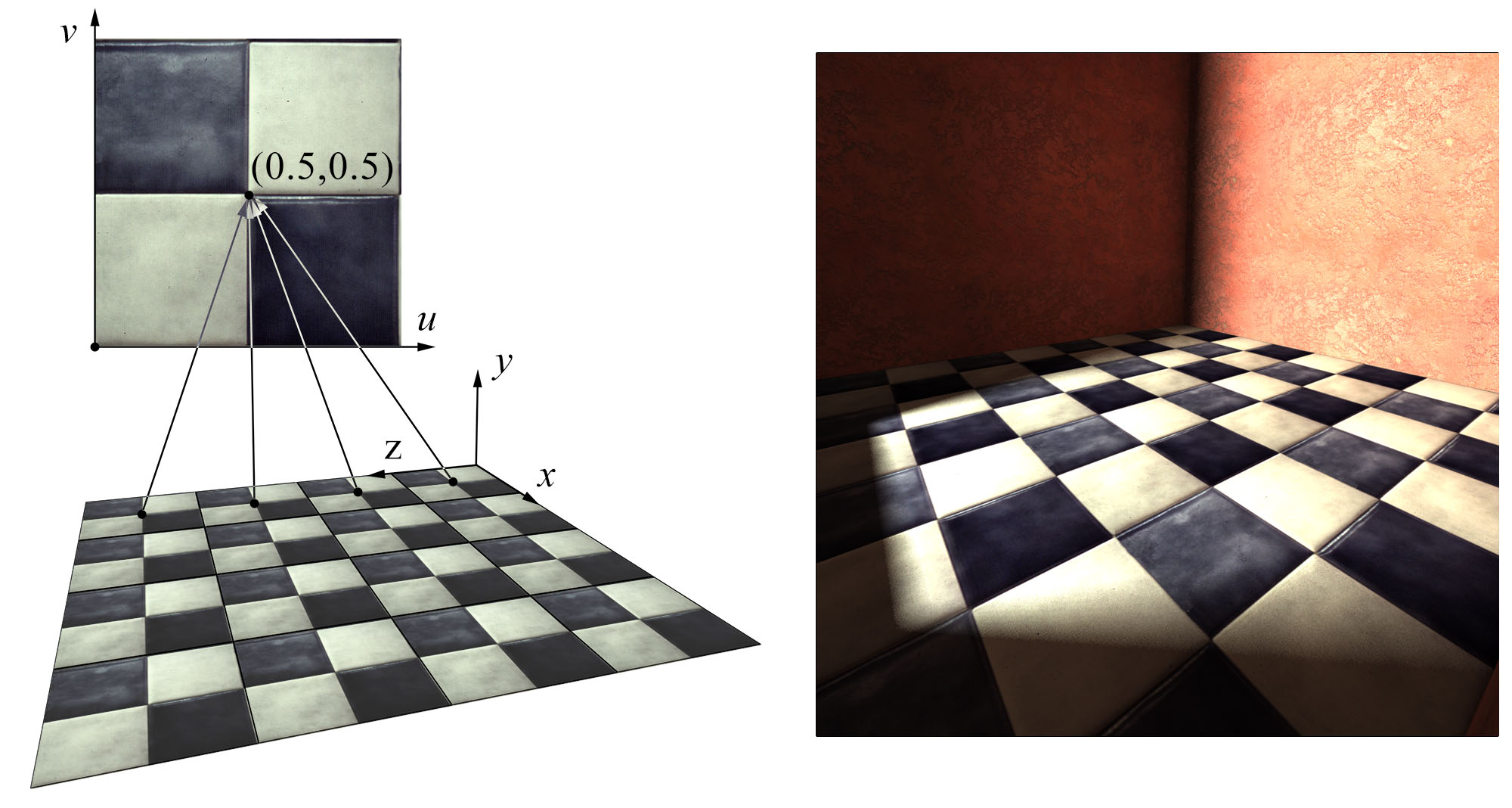
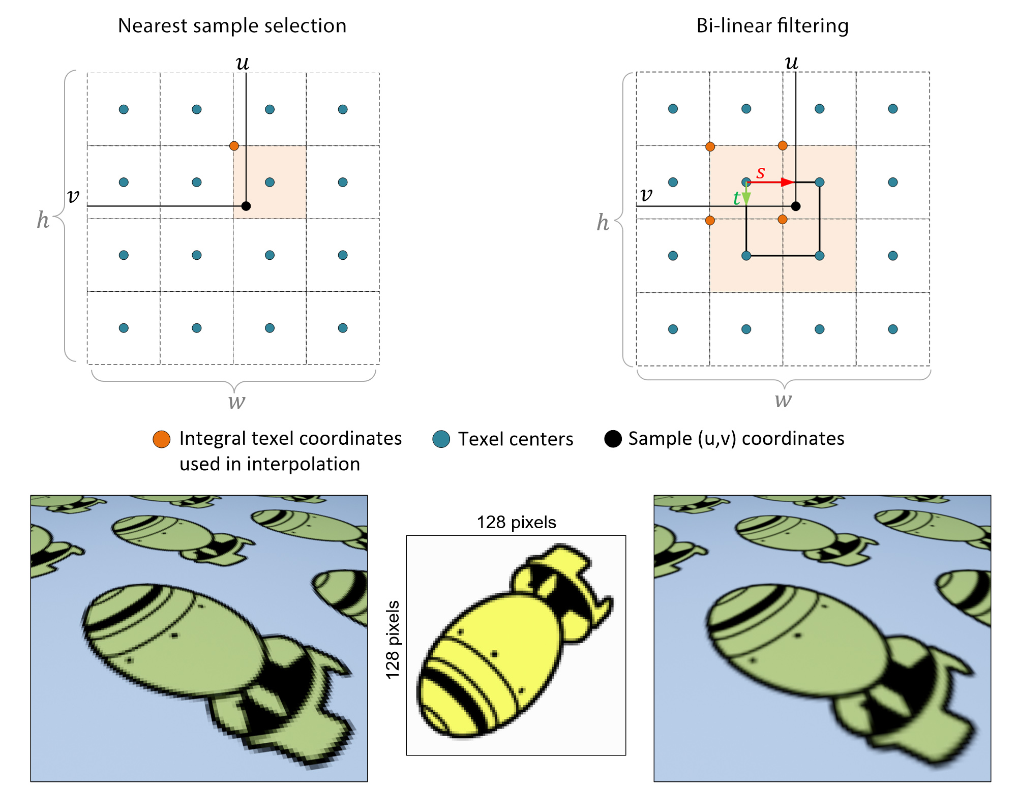
Given the set of texture coordinates, a shading algorithm must determine the value of the texture at that location on the texture map. The simplest way to do this is to choose the closest texel. Bear in mind that the texture coordinates $(u,v)$ are eventually mapped² to the normalized $[0,1]$ interval prior to fetching a value from the texture map, while the stored texture has an specific width $w$ and height $h$ in pixel units, e.g. 512$\times$512. Therefore, to obtain the desired pixel location $(i,j)$, the texture coordinates are scaled by the corresponding size of the bitmap. The resulting values are not integers in general, since $u$ and $v$ can take any value between 0.0 and 1.0. The "nearest" texel is decided by rounding the scaled parameters $u\cdot w$ and $v\cdot h$.

However, as demonstrated in the following figure (left), when the texture coordinates of multiple samples on the polygonal surface are eventually mapped to the same nearest texel on the texture map, we have a situation that is called texture magnification and there is when pixelization occurs. The bitmap texels are visibly magnified in view, resulting in an often experience-breaking visual artifact. This is due to the fact that the sampled information on the texture is fixed and limited while the magnification resulting from the projection of the textured geometry is not. The texture simply has no more detail to sample and visualize. We usually attempt to alleviate the problem by performing some form of filtering that cannot of course increase the fidelity of the texture, but can rather smooth the texture values. The typical way to address the problem is to look up more texels in the vicinity of the texture coordinate location and perform a weighted average of them. The most common way to do this is bilinear interpolation of the four neighboring texels; the contribution of each texel is weighted by the proximity of its center to the sample location.

Texture Minification

When texture-mapped surfaces are projected in such a way that a single image sample corresponds to multiple texels in the texture space (see figure below), the texture is under-sampled and the textural information cannot be properly reconstructed, leading to serious and quite noticeable aliasing artifacts, severely impacting the image quality.

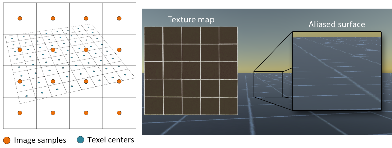
Clearly, this is typical case where the requirements of proper sampling in order to ensure correct signal reconstruction no longer hold (see sampling theorem ³ ). To be able to correctly sample the texture, instead of selecting an arbitrary texture sample within the image pixel area, one should take into account all texels that are projected within the pixel area, using some form of averaging filter. However, an averaging operation corresponds to a frequency limiting filter applied on the texture. In other words, averaging the texels subtended by the pixel, intentionally lowers the detail of the textural information so that it can be sampled using the (lower) sampling rate of the image and correctly reconstruct the visible information.

The filtering operation itself is problematic, however. When texture minification occurs, a pixel may cover an area ranging from a few texels up to the entire image, meaning that a texel average calculation may include a difficult to predict area on the texture, with an arbitrarily large number of pixels, rendering exact filtering impractical. What is done instead is pre-filtering. The texture image is filtered with a smoothing filter of increasing yet predetermined size. Every texel of a filtered version of the texture corresponds to a pre-calculated weighted average at the same location on the original image. To reduce storage, each filtered version is smaller than the version preceding it in terms of filter size, as shown in the following figure. This is a reasonable approximation, given that the smoothing effect of the filter reduces the detail of the texture. This pre-filtering operation, called mip-mapping ("mip" from the Latin "multum in parvo" — many things in a small space), is typically performed offline, during texture preparation and loading.

Isotropic Filtering

At runtime, the most appropriate level of pre-filtered texture detail (mipmap) is selected, based on an approximate estimation of the pixel coverage area in texture space (see figure above). This can be determined very fast, provided the image-space derivatives of the texture coordinates are available, which is true in the case of the triangle rasterization pipeline. Selection of a mipmap level may not be "snapped" at distinct pre-filtered images. Instead, we can allow the texture filter size to take arbitrary, continuous values, whose integer part determines the closest two mipmap levels and the fractional part an interpolation factor between them. In effect, such a mode of texture access performs a "tri-linear filtering": bilinear filtering is used within each mipmap to determine the values at the sampled location (see texture magnification), followed by another linear interpolation to mix the closest pre-filtered texture versions.

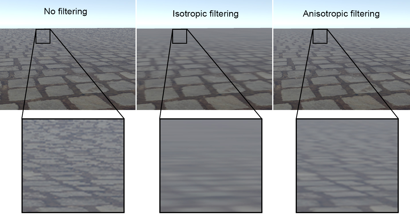
In its simplest and most compact form, the pre-filtered texture is processed using a 1:1 filter kernel (e.g. square), assuming the projection of the image pixel on the texture space is a compact shape. This process is called isotropic filtering. However, this is often not the case, as the texture area covered by the pixel can be elongated or tilted. In those cases, and to avoid aliasing, the filter kernel size is overestimated, resulting in a blurry appearance of the textured surface, as shown in the middle inset of the following figure.

Anisotropic Filtering

To resolve the overestimation of elongated and arbitrarily oriented smoothing filters, the respective filter kernel must be anisotropic in terms of aspect ratio and able to match an arbitrary orientation in the texture space. Explicitly defining all such configurations and generating the corresponding pre-filtered texture versions is impractical. Instead, anisotropic filtering approximates an elongated filter kernel by arranging multiple isotropic filters in a line and computing their weighted average. This means that for a single anisotropic texture fetch, multiple isotropic texture filtering operations must be performed, rendering the approach more expensive than simple isotropic minification filtering. However, texture filtering results are significantly improved, as demonstrated in the right inset of the following figure.

Procedural Textures

As mentioned earlier in this section, image-based texturing is the most comprehensive and natural way to apply a texture that is stored in an array of pre-recorded or computed discrete values. There are many cases however, when a surface (or volume) attribute can be directly calculated from a mathematical model or can, in general, be derived in a procedural, algorithmic manner. The procedural texturing does necessarily make use of an intermediate parametric space. Instead, it may directly and uniquely associate an input set of coordinates with an output texture value. Procedural textures can be considered as time-varying self-contained systems and are often referred to as procedural shaders, i.e black boxes that can be linked together to process a set of input coordinates and modify a material attribute of a surface or volume. A procedural texture can be used to calculate a color triplet, a normalized set of coordinates, a vector direction, or a scalar value. Procedural shaders can also implement mathematical or logical operations to facilitate the combination of texture maps and procedural textures into shader hierarchies (see next).

An important question to pose is why somebody should use procedural textures instead of parametric image maps. In order to explain this, we need to examine the properties of a procedural texture. First, by definition, a procedural texturing system operates on continuous input parameters and generates a continuous output of infinite resolution (constrained of course by the numerical precision). This means that sampling a surface at a high resolution will not yield a blurred version of some interpolated discrete data, as is the case with the bitmap-based texturing, but a finer version of the output domain. Therefore, procedural textures do not suffer from magnification problems. Second, directly mapping Cartesian coordinates as the input to a 3D procedural texture leads to a texture that is distortion-free, as no intermediate parametric representation is involved, which may introduce mapping singularities and stretching. Last, the procedural textures can (and should be) defined in a way to ensure a meaningful mapping from the entire spatial domain to the output domain.

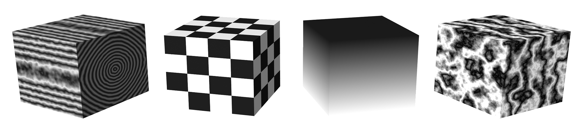
In nature, many periodic patterns, self-similar shapes or chaotic and noisy signals can be very accurately modeled using procedural textures at an arbitrary sampling rate. Their ability to mathematically control the appearance of the generated pattern with the proper selection of texture modeling parameters, provides a useful visualization tool for artists and scientists alike.

Procedural textures can be driven from geometric features, computed either at runtime or as a pre-processing step, such as curvature and or surface elevation or orientation. In the example of the following figure, multiple procedural textures are blended together using the pre-computed curvature and visibility (ambient occlusion) of the surface as blending factors, in order to achieve a weathering effect on a painted metallic surface.

Two common procedural textures that are often used in conjunction with a simple mathematical function, such as a sine, are Perlin noise and $1/f$ noise. Perlin noise is a smoothly interpolated field of pre-computed random values laid out on a uniform 3D grid. The grid is considered infinite and stored random values are indexed by some coordinate hashing function that remaps arbitrary grid node locations to a set of predetermined, known ones. Compared to a typical random number generator, Perlin noise exhibits certain desirable characteristics for graphics, including consistency, deterministic behavior, bounded frequency (maximum detail) and smoothness.

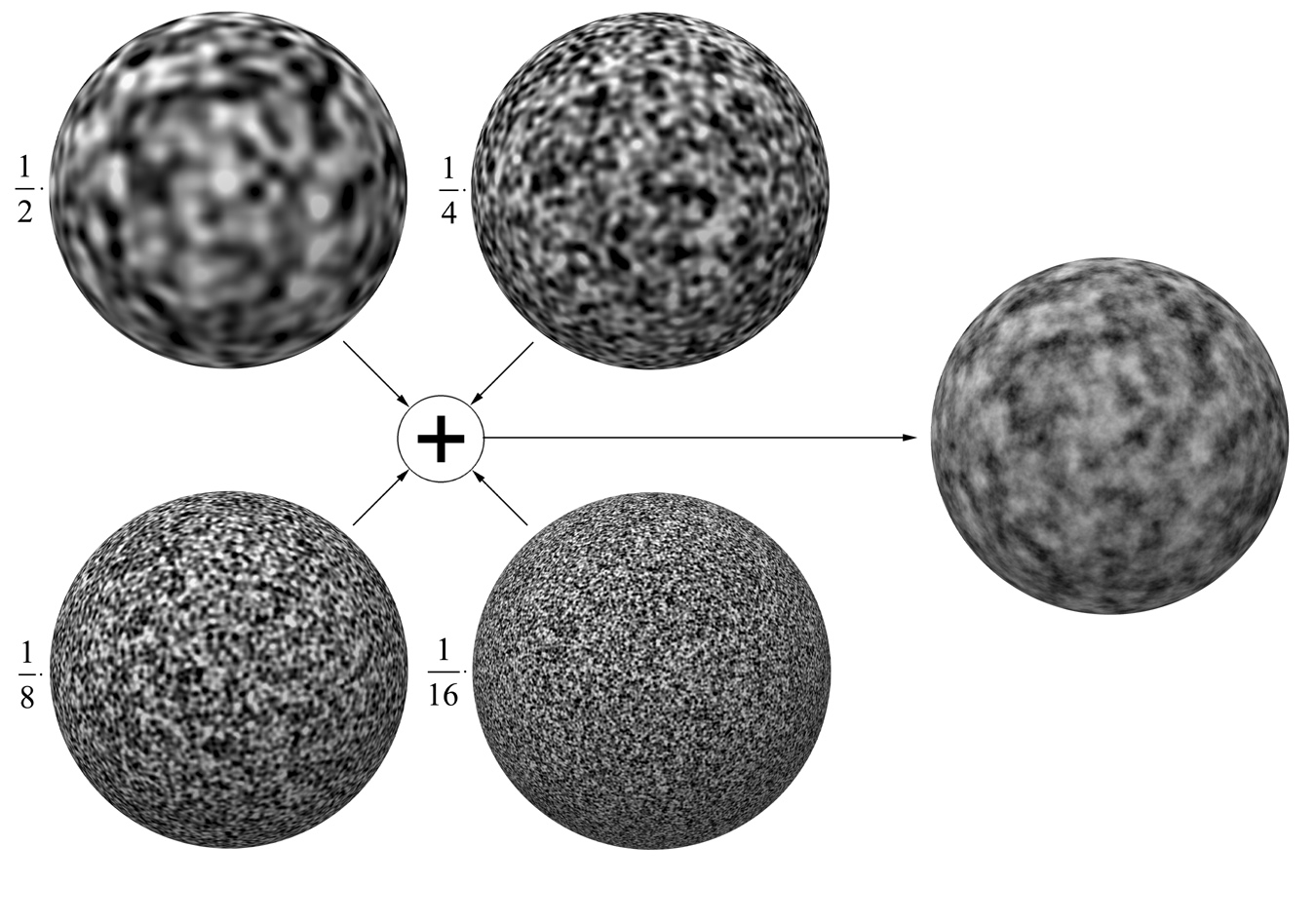
$1/f$ noise is a recurring random pattern in the physical world. It is simply the superposition of random patterns of increasing detail. However, the more detailed the pattern, the smaller its contribution to the final pattern. More precisely, if $f$ is the detail level (maximum frequency) of the random pattern, its contribution to the $1/f$ noise is inversely proportional to $f$, hence the name. Grainy materials, smoke and turbulent media can be efficiently represented in high detail using $1/f$ noise, by overlapping Perlin noise at different scales.

Texture Transformations

Texture coordinates or other coordinates that are used for the indexing of an image-based or procedural texture can be transformed, prior to being used for texture mapping, in the same spirit we apply transformations to modify or model 2D and 3D space. Therefore, any geometric transformation or projection can affect the texture coordinates, such as scale, rotation, translation or perspective projection. This is useful, in order to control the exact mapping precisely or change it over time. For example, if we want a texture pattern to repeat twice as many times over a surface as it was its initial mapping, we can multiply each texture coordinate by 2 prior to indexing the texture image. Therefore texture coordinate transformations are very often used to control texture tiling and orientation. Another typical example is the translation of a texture coordinate using a time-dependent offset to make a texture shift over time. This is an easy way to model flowing water or the motion of a conveyor belt.

Texture Hierarchies

Texture images can provide local control and definition of non-principled shapes whereas procedural textures can offer high precision and global control. It is therefore often the case that we combine the strengths of individual texture types to implement more complex shaders, by hierarchically connecting image-based and procedural textures in a directed acyclic graph, as shown in the following figure. Upon a texture mapping request during shading, the output of one texture node in the graph is used as the input (parameterization) to the next and so on, until the final texture value (the root of the directed graph here) is resolved.

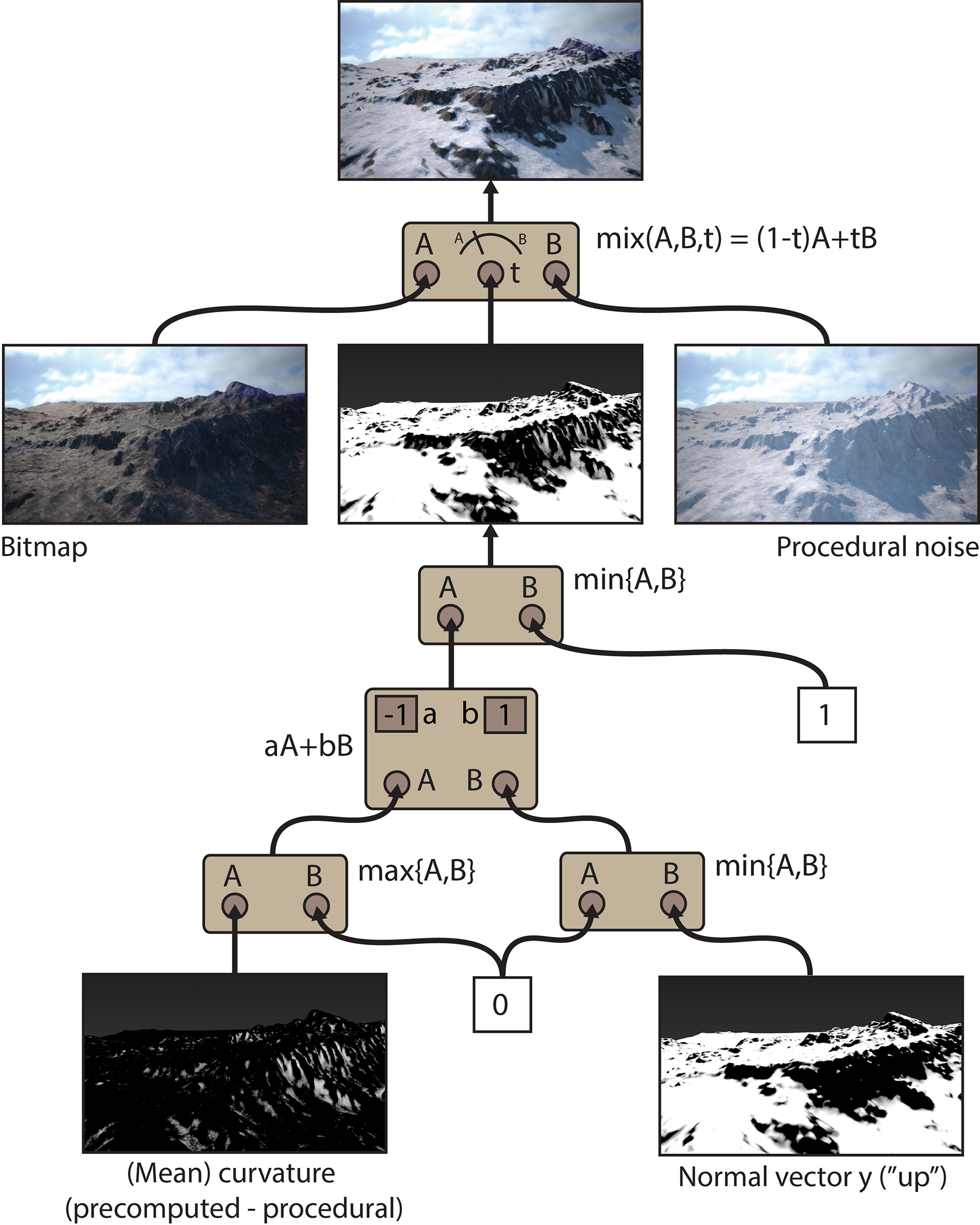
In this particular example, we create a "snow mask" to blend between a rock texture and a snow texture. The Snow procedural color should be applied on shaded points that a) face upwards, towards the falling snow and b) are trapped in deep recesses and are slower to thaw or make difficult for chunks of snow to fall off. A surface feature, the mean curvature for a particular radius has been pre-computed and stored in a texture atlas, with negative values corresponding to recesses and positive values to protrusions. The positive values are clamped to zero via a max operator. Next, we use the Y value of the surface’s normal vector (negative values clamped to zero) and the results of clamped curvature and normal Y are added together, using a simple linear combination mathematical operation node, which we can treat as a procedural element. We retained the negative values of mean curvature, which represent recesses on the surface and therefore they contribute here to the intended "snow" mask after inverting the sign (see -1 parameter on the graphical representation of the node). The result, is clamped to 1 by connecting it with a constant value (1) and can now be used as a linear blending coefficient between a texture image (rocky ground) and and a procedural noise shader (snow) to produce a realistic deposition of snow on a mountainous landscape.

Representing Geometric Detail

When modeling a surface, one may not include all minute details, or these details may need to be decided later on. Additionally, it is often the case that a 3D model with too much geometric detail is too heavy to be rendered at the desired display performance, memory budget, or both. In all these circumstances, we need to represent and display geometric detail at runtime, in some form of texture mapping operation. In the following sections, we will examine ways to achieve this, with varying degrees of fidelity and cost.

Displacement Mapping

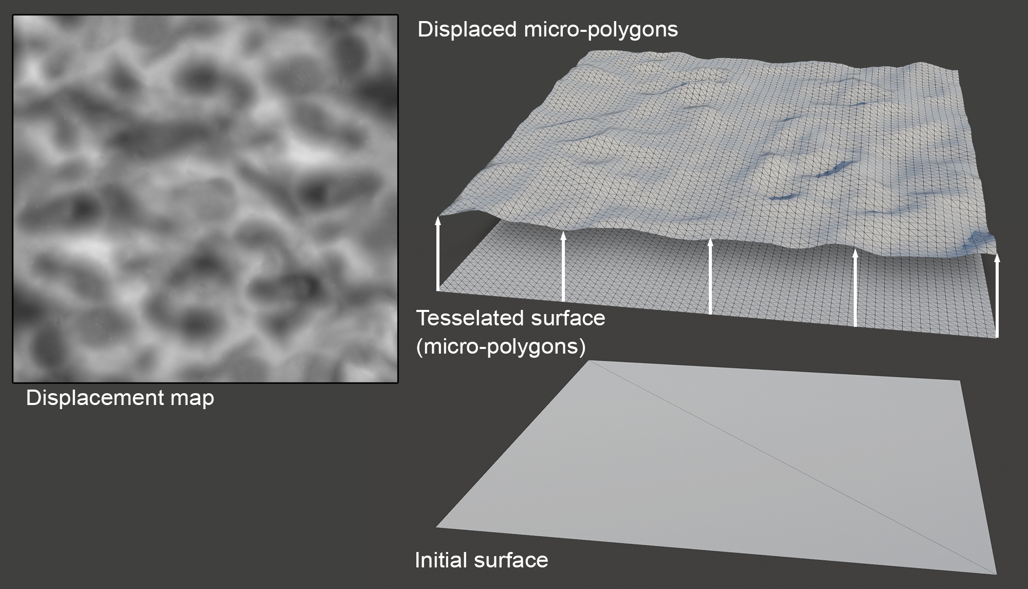
Displacement mapping creates relief patterns on a surface by moving the vertices along the original surface normal direction or along a predefined vector according to the intensity of the texture evaluated at each point. The elevation texture is a scalar height field representing the relief pattern, called displacement or height map. Needless to say, since the displacement map carries an elevation pattern that is far more detailed than the intrinsic geometric structure, it the latter is incapable of deforming in any meaningful way to match the displacement map’s definition. Therefore, during rendering, the original geometry is temporarily subdivided to match the lowest sampling rate between the screen space and the texture space, while filtering the height map as per typical texture minification.

The big advantage of displacement mapping over the other method that will be discussed next, is that it truly generates a pattern in relief and not a shading illusion. This means that the textured surface exhibits the proper parallax effect from all viewing angles and at all surface locations, including the object’s silhouette. On the downside, the highly detailed surface it requires makes the technique unfavorable for real-time rendering of relief patterns. Displacement mapping is used in real-time applications in conjunction with specialized hardware tesselation and micro-polygon data structures, but it is generally more widely applicable in offline rendering.

Normal Mapping

An important observation, which is the key idea behind normal mapping, a low-cost detail mapping technique, is how the relief pattern is finally perceived by the human eye. When we look at a bumpy surface, what we actually deduce the shape of the relief pattern from most of the time, is the variation of the surface illumination, which is the result of the surface shading. Now recall from the local shading models that the only local surface attribute that contributes to the shading calculation is the normal vector itself and no other “elevation” information. This has the amazing implication that we can have the same local visual effect of a geometrically wrinkled surface by directly calculating how the normal vector would be perturbed, if the surface was elevated, but without actually moving the surface points. This way, the eye is tricked to believe that the three-dimensional model is substantially elaborate in terms of geometry, whereas we only alter the normal vector in the shading calculation.

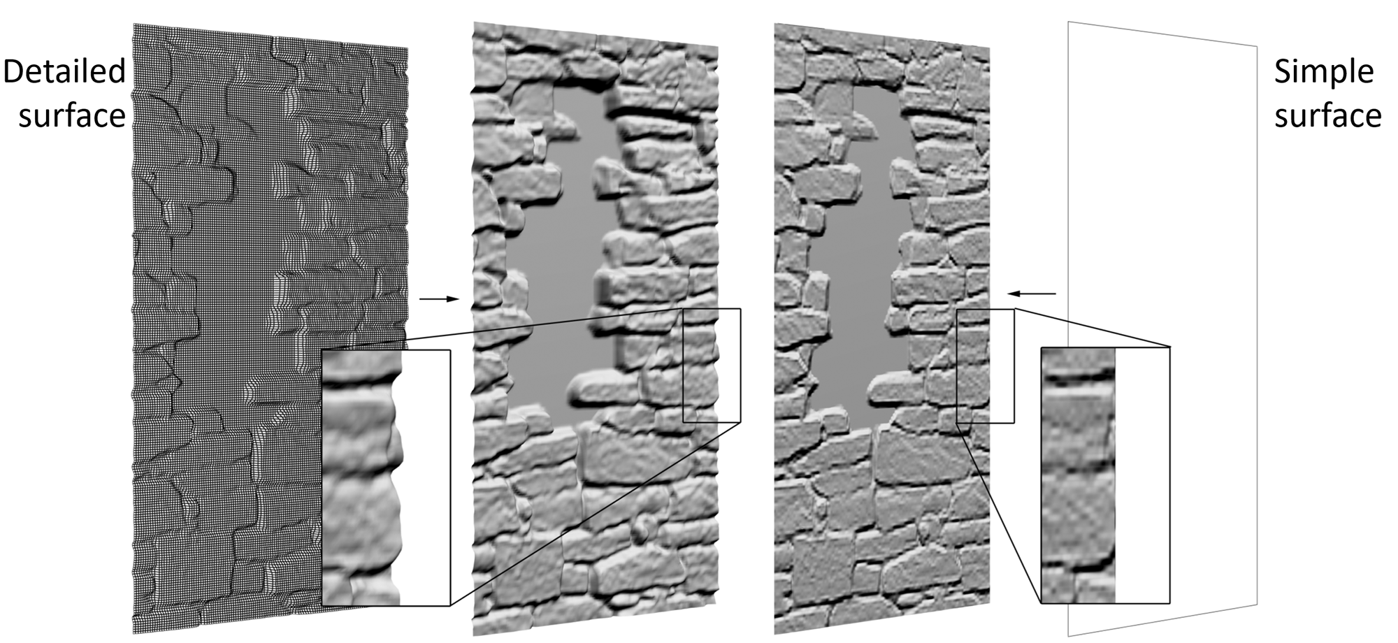
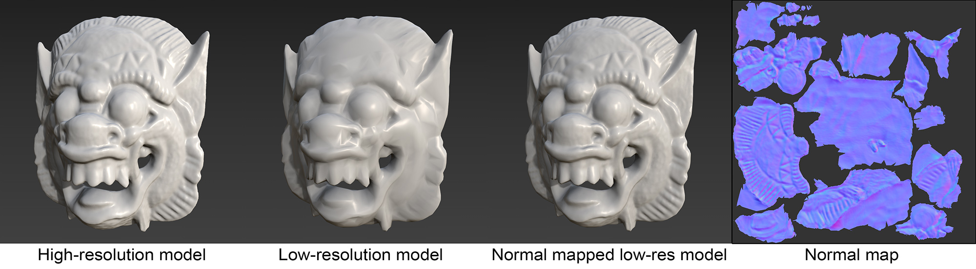
The following figure shows a comparison between a displaced surface and a normal-mapped one. The displaced surface needs a fine tessellation in order for the vertices to be able to track the texture-space offset variations. The resulting, displaced mesh correctly captures the relief details and is accurately shaded and clipped across the whole surface. On the other hand, if the same texture information was applied as a normal map to the surface, there would be no need for any tessellation of the polygons. A very simple geometric representation could be used and still produce a good approximation of the shading on the surface. However, this otherwise convincing shading trick has two disadvantages. First, the representation of relative offsets is poor, when deep depressions are present in the elevation pattern. Shading alone cannot stand in for the occlusion one raised part of the displacement would cause to parts of the elevated or depressed geometry behind it, with respect to the given point of view. The other problem occurs at the surface edges, where due to the fact that the geometry is not actually bumpy, the shading conflicts with the clean, smooth surface silhouettes.

The most common way to represent and apply the "replacement" normals on a surface is tangent-space normal mapping. To understand how tangent-space normal maps are defined, let us first describe the notion of a target-space coordinate system. We already know about the normal vector of a surface, which is a unit-sized vector always perpendicular to the surface at any point, pointing outwards. Let us consider a local 3D reference frame, whose one axis is the normal vector. The remaining two axes are by definition of an orthogonal coordinate system perpendicular to the normal vector and therefore parallel to the surface at any given point. We can now freely choose any two other vectors, orthogonal to each other on that tangent plane to act as the remaining two axes of the tangent-space coordinate system. In practice, by construction, these vectors, the tangent and bitangent, are chosen so that they conveniently follow an as smooth as possible vector field developed on the surface. Typically they follow the texture coordinates. For polygonal meshes, tangent vectors are stored as additional vertex attributes on mesh vertices, along with the vertex shading normals. The tangent space is defined in such a way that the local z direction points at the (unperturbed) interpolated normal vector, the x direction coincides with the tangent vector and the bitangent vector is parallel to the local y axis.

Tangent-space normals are versatile and convenient for modeling since they are immune to transformations and deformations and the corresponding normal maps can be used as tiled textures on an arbitrary surface. The normal maps store the x, y and z coordinates of the replacement normals in tangent-space coordinates, by typically mapping x (tangent) to red, y (bitangent) to blue and z (original normal) to blue. Since the new normal vector is not expected to be inverted with respect to the original shading normal, no negative coordinates are assumed for its z value and the coordinate is stored in higher precision (only positive values mean one more bit for arithmetic representation). Tangent and bitangent coordinates however can be both negative or positive, depending on the direction the replacement normal is "bent" on the tangent plane. The typical mapping from a tangent-space normal $\mathbf{n}=(n_x, n_y, n_z)$ to a normalized RGB triplet (values in the range 0.0 to 1.0) is:

$$R = \frac{n_x+1}{2}, G = \frac{n_y+1}{2}, B=n_z$$

An example of a normal map can be shown in the following figure, right inset. Tangent-space normal maps have a distinctive "bluish" color. This is due to the fact that statistically, the normals stored are pointing towards the true normal of the surface on average, which in RGB encoding corresponds to the value (0.5, 0.5, 1.0), i.e. light blue.

Detail Baking

When we have a high-resolution 3D model of an object that must be simplified for practical rendering or geometric processing, we can extract the geometric elevation or surface direction variations from the high-resolution model version and map it onto the low-resolution model during rendering, either as a displacement map or as a normal map. This way, although the polygonal model is simplified, we can still visualize its details with sufficient fidelity to be used in interactive rendering applications.

The general process to produce a normal or displacement map from a high-resolution model is the following:

• Provide a simplified version of the high-resolution model, either via simplification of the original model or via a proxy 3D model generated independently. In the latter case, the two object versions must be properly scaled and aligned.

• Provide an existing or build a new texture parameterization with unique, non-overlapping texture coordinates for the low-resolution model to build the detail texture with, at a user-defined resolution.

• For the surface positions corresponding to each detail texture texel, sample the corresponding point(s) on the detailed geometry and measure the detail feature at hand. If surface elevation is stored as the detail information, measure the signed distance from the low-resolution mesh to the high-resolution one. If surface direction is stored as a tangent-space normal map, obtain the high-resolution surface normal and encode the deviation from the low-resolution shading normal. Correspondences between the surfaces can be established in different ways, but the most reliable way is to trace rays from the low-resolution surface along the normal direction and register the closest hit.

• Post-process the gathered data to smooth/normalize the data. Elevation measurements may require a remapping to positive distances and normalization.

Lighting

Emission and Light Sources

As mentioned in the introductory material, any image synthesis task that attempts to simulate or imitate how objects appear in the physical world, needs to also describe the energy that is provided to the virtual environment, which the various geometric element and their materials interact with and whose captured response on the virtual image sensor(s) forms the final image, according to a rendering pipeline. Even for non-physically-based rendering tasks, such as illustrative rendering and data visualization applications, one or more assumed virtual lights are present in order to provide shading variations on the 3D data that are rendered.

In principle, any point on or within every body represented in the virtual environment, be that a surface boundary representation, a volumetric medium or an all-encompassing, distant scene boundary, can be light emitting, since this is what happens in the physical world. This means that energy in a virtual environment can be contributed by any geometric element and we must therefore ensure that a proper light sampling mechanism is established to gather that energy consistently (see also rendering unit). However, for practical reasons and to simplify the assumptions and sampling process, we typically specify a separate set of individual light sources to act as the energy providing elements of our virtual environment. In more advanced rendering architectures supporting path tracing and statistical many-light rendering, we can also account for the contribution of arbitrary emissive surface locations, typically defined by emissive information on textures (emissive textures).

Types of Light Sources

Local vs Distant Light Sources

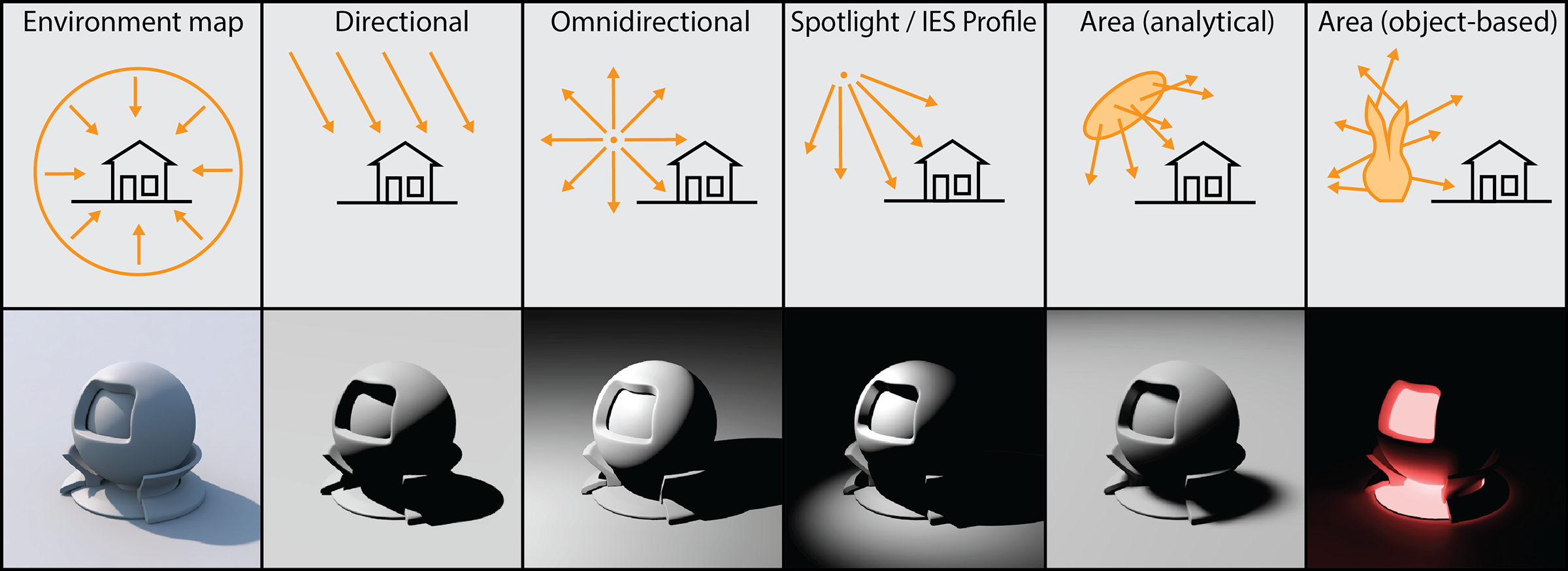
Light sources can be broadly categorized according to how they are defined and what is their relationship with the virtual environment. At a high-level, we can distinguish lights as local and distant. Local light sources represent mathematically defined luminaires that can be positioned within the environment at precise locations, or the emissive bodies or surfaces of geometric elements of the scene. For these light sources, the emission characteristics represent what light these elements output at the source, i.e. at the locations of origin on their geometry or position in space. The incident light contribution of these sources on the lit geometry is then estimated using the appropriate light transport equations, usually involving the attenuation of energy as it disperses through space.

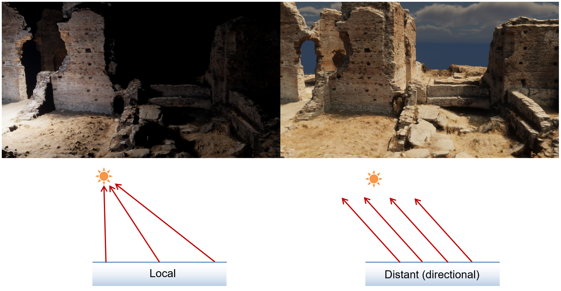
On the other hand, distant light sources model light that enters the virtual environment from a very large distance compared to the extents of the scene and from contributing emissive bodies or dispersion through media that cannot be modeled in the scope of or extent of the geometric elements at hand. Prominent examples of such distant lights are sunlight and the illumination from captured or modeled distant environments, such as sky dome illumination and 360$^{\circ}$ panoramic images of the scene’s surroundings (see environment maps below). Sunlight, as observed from a vantage point on earth, can only be measured at the point of incidence, and given the vast distance to the sun compared to distances in the virtual environment, this measurement does not practically change. Furthermore, given the relative scale of things, rays from the sun appear to hit the scene almost parallel to each other. This is why we typically model such a source as a directional light, meaning that we do not define its location, but rather a direction that the light comes from, which is identical to all shading computations involving that light, no matter where in the scene the shaded point is located (see figure below).

Punctual vs Area Light Sources

In reality, all emissive bodies have some mass and occupy a certain volume of space. In this sense, the only realistic light sources are area lights (including distant spherical emitters, see next figure). Evaluating the lighting from such a luminous body requires some form of analytical or numerical (statistical) evaluation of their contribution from their entire domain (surface, volume or domain of directions), something that may be too demanding or prohibitive for certain practical scenarios, such as real-time rendering. Very often in computer graphics we simplify things by inventing simpler approaches in terms of formulation and evaluation, and lighting is no exception. In many practical rendering implementations, light sources can be punctual, in the sense that all light is emitted from a single point in space, with no volume or surface. This greatly simplifies outgoing light evaluation as it eliminates the need for illumination integration or sampling. Furthermore, it simplifies the evaluation of light source visibility, making the problem tractable for interactive applications (see shadows below). In most interactive applications, where real-time graphics are involved, light sources are typically configured as point lights, directional punctual lights or "spotlights", i.e. punctual emitters with a constrained, conical lobe of emission. In non-rasterization-based rendering however, all types of light sources are usually supported, since light transport is stochastically evaluated, seamlessly integrating light sampling in the process.

Describing Light

Basic Quantities

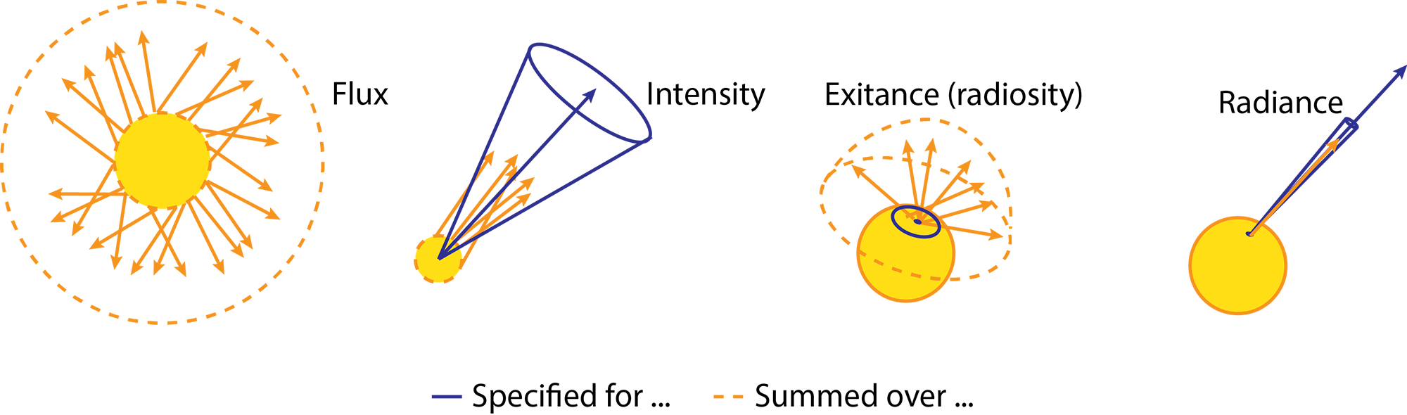
Light-emitting bodies provide energy to the environment in the form of electromagnetic radiation in the visible spectrum, which can be quantified and measured in standard energy units, such as Joules (in the SI system). However, describing a process using energy is not meaningful as energy is constantly converted to and from light, piling up. Therefore we cannot successfully describe a steady state of emission and light transport using energy. However, if we consider the rate of energy emission, absorption and scattering, that is, energy over time, this describes energy exchange in a steady manner. The rate of radiant energy provided or expended over time is the radiant power or radiant flux $\Phi$, measured in Watts (W) in the SI system. We are also often interested in describing or knowing how much of the light power exiting or entering a point is concentrated in a particular conical beam. This is called radiant intensity and is expressed in Watts per steradian. A steradian is a a the unit of a dimensionless quantity called a solid angle, which describes the opening of a beam in space and is the three-dimensional counterpart of an angle in two-dimensions.

As we will discuss next, flux and intensity are commonly used for describing the emissive characteristics of light sources. However, there is another radiometric quantity that is important to graphics, radience $L$. Radiance describes the amount of light exiting or entering an infinitesimally tight spot around a point and traveling within a very tight beam in space. It is important to the modeling and estimation of light transport using geometric optics, because at the limit, it allows to represent how much light travels on a linear path segment connecting two points in space or carried by a specific ray of light. Typically, the light entering or exiting a surface is affected by the flow of energy through a given "opening" locally oriented parallel to the surface. However, when measuring radiance, we always consider light crossing the surface with maximal flow, thus factoring out the actual flow of energy through the surface and focusing on the radiant energy that traverses the space above the point of incidence/exitance.

The fourth radiometric quantity that is important for computer graphics computations, especially when measurements are considered, is irradiance and its symmetric quantity for outgoing light, radiosity. Irradiance represents the sum of all radiant energy hitting a particular infinitesimal area around a point in a surface coming from all possible directions. It answers the typical question "how much light does a surface point receive". In calculations, it is the integral of all radiance incident on a point of interest over all directions that the point can potentially receive light from, i.e. either the hemisphere above the point or the spherical domain of all possible directions, including illumination transmitted from within the body of the material.

It is important to clarify here that so far, we have described quantities that regard emission and transmission of energy in the entire spectrum of electromagnetic radiation. However, when representing interactions of visible light, only a limited range of wavelengths must be accounted for. Furthermore, the human eye photoreceptors have different response to the different wavelengths of visible light, their response weighing and blending the wavelengths of visible light in a non uniform manner. For these reasons, a different field of study of luminous energy has emerged, photometry, which defines equivalent quantities to the radiometric ones, adjusting their values to the response of the human visual system.

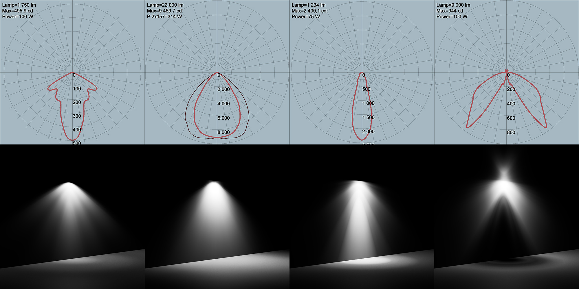
The equivalent photometric quantity to describe power is luminous flux, measured in lumens (lm). Similarly, luminous intensity is the photometric equivalent of radiant intensity and again it represents the emitted or transmitted luminous power per solid angle. Considering that luminous power is measured in lumens, luminous intensity is measured in lm/sr, or candela. Luminous intensity regards the directional contribution of power and it is used in the definition of luminaires, and more precisely, in the specification of the photometric web for real light sources, i.e. a chart that contains the measured luminous intensity according to illumination direction relative to the light source. See more details in the definition of light sources section below.

The photometric equivalent of irradiance is illuminance and is measured in lux (lx). 1 lx is 1 lm per $m^2$. Illuminance measures how much light reaches a particular point on a surface, aggregated over all directions. There is of course defined the symmetrical term for outgoing light (exitance), the luminous exitance of a surface.

Let us now provide a crude but effective example about the relation between radiant and luminous quantities. Imagine an electric light bulb plugged into a socket. The bulb has a specific power consumption, say 50W. This is not the radiant power of the bulb however, since a lot of the electric energy is converted to heat. The ratio of the consumed power that is given off as emission in the entire spectrum determines the electrical efficiency of the bulb as an electrical device, i.e. how much input power is converted into something useful. With an efficiency of 50%, such bulb would convert 25W to radiant power and 25W into heat. However, if we asked how much of the useful energy converted by the bulb ends up in the visible spectrum for human beings, then we would also use the light bulb’s luminous efficacy to determine that fraction in lm. Since this is a conversion rate for energy, it is bounded and the maximum value is 683 lm per W of radiant power. Practical realistic lighting elements have a lower luminous efficacy, of course. Another way to define luminous efficacy is with respect to the initial, input power. Again, even very efficient LED lights have a conversion ratio of about 200lm/W.

Defining Light Source Emission

According to the definitions of photometric quantities, in a physically-correct rendering pipeline, it is common to describe virtual light sources using the most suitable specification, interchangeably. When directional aspects of lighting are important for the application, i.e. how much light is emitted in a particular direction, intensity is often the quantity of choice. When simulating real luminaires (lighting system elements), graphics simulations may read and adjust the light source’s directional emission according to a photometric web profile. This diagram, associates luminous intensity with a particular emission direction, as shown in the following figure. The Illuminating Engineering Society (IES) has defined a file format, the IES profile, which describes a light’s distribution from a light source using real world measured data.

The light sources are also characterized by their emission color. In the majority if rendering software, luminous power, or any other quantity that determines how bright a source is, is decoupled from the colorization of the source for reasons of detailed control. Color of a light source can be provided either as color temperature, if the intention is to model real bulbs, and/or in the form of a filter color that modulates "white" emission.

Environment Lighting

So far we have examined sources of illumination that are local in nature. However in real environments light also comes from distant luminous bodies or scattered on surfaces or within participating media, whose distance or extent are of a far greater scale than the geometry to be rendered, such as the sky dome. To account for such illumination in a lighting simulation and therefore image synthesis task, we may collectively refer to that kind of "distant" illumination as environment lighting, although we will specialize the category further.

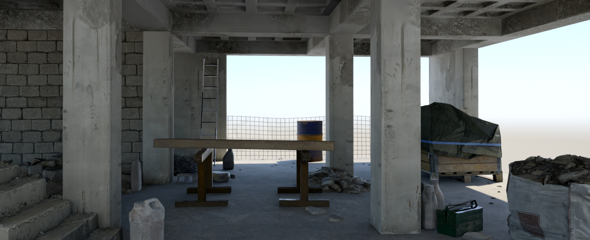
When rendering virtual environments, we must also consider two related problems: First, not all visible entities in a synthetic image are actually represented by geometry. For example, in an outdoor scene, a distant mountain range and a cloudy sky can be considered as a combined distant spherical object that surrounds and completely encases our virtual world. This is important both for efficiency reasons but also for bounding the scope of our work to elements that we are actually going to closely inspect or interact with. Second, in many situations we are asked to integrate visual material of real physical spaces with computer generated graphics. Embedding a virtual object in a live action scene for a feature film or using a photographed panorama as an environment for inspecting a 3D model are two typical such examples. In both cases, simply blending the two visuals is not enough. Lighting from the real environment representation must also affect the virtual entities, so that the latter "fit in" into the environment.

In terms of modeling environment lighting the same principles as querying directional light sources apply; we assume that the environment is so distant (and expansive), that all addressable locations in the virtual world are mapped to the same location on the environment for a specific look up direction. In other words, the environment is only indexed by direction.

Environment Maps

An environment map is simply a digitized or computed panoramic representation of incoming light, parameterized by illumination direction. Since the environment map is a digital image, a mapping function must be defined between the spherical domain of all potential directions to the parametric space of the image. There are many ways to map a 2D surface to a sphere and vice versa and this has been an important part of map making for many years. It can be shown that any mapping from the plane to the sphere introduces either area or angular distortion. Applications are tasked with choosing a mapping that best fulfills their requirements.

Latitude - Longitude Maps

Latitude - Longitude environment maps simply map texture coordinates to the polar coordinates of the look-up direction, i.e. elevation (latitude) and azimuth (longitude). This is probably the most intuitive mapping function between the spherical domain of unit directions and the rectangular texture space. Single-image lat/long environment maps are easy to find and use in most applications, since the indexing of the texture map is straightforward.

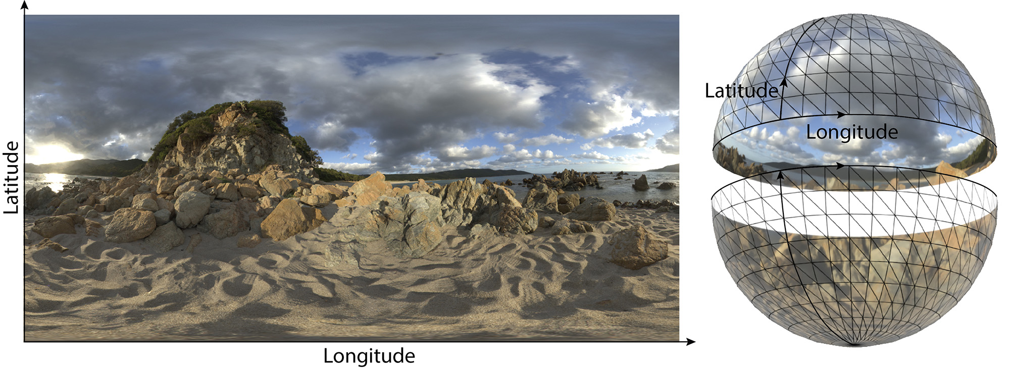
However, lat/long environment maps are not area-preserving, with the density (pixels per unit area) increasing towards the poles and resulting in a singularity at the extremes, where the map values are not dependent any more on the longitude. The resulting stretching has lead the computer graphics community to seek more appropriate mapping functions for the storage and access of environment map data.

Cube Maps

One of the most successful mapping method for indexing image information based on direction vectors is the cube map. The cube map is an arrangement of 6 equally-sized square maps positioned on the sides of an imaginary cube, which is centered at a user-specified location in space. The center of the cube map is used as the center of projection to form 6 independent projections, each one subtended by one of the sides of the cube. By construction, each projection is a symmetrical perspective projection with an aperture of 90 degrees. The complete spherical environment surrounding the center of projection is then mapped to the sides of the cube map. Going from a direction to a location on one of the 6 planar textures corresponding to the cube map sides (sub-textures), one first determines the projection side, according to the sign and axis of the largest absolute direction coordinate (e.g, +X). Then, the vector is perspectively projected on the chosen side, by dividing the remaining vector coordinates by the dominant one. The resulting coordinate pair is normalized to the square texture window.

There are several benefits in using a cube map instead of a lat/long texture map. First, the cube map exhibits no singularities. Second, area distortion is smaller. Finally, a cube map, practically consisting of 6 perspective projections, can be easily created using the rasterization pipeline from within a running interactive application, thus being able to capture an environment map from computer generated content, without requiring more expensive techniques such as ray tracing, in addition to being inherently compatible with any other rendering technique.

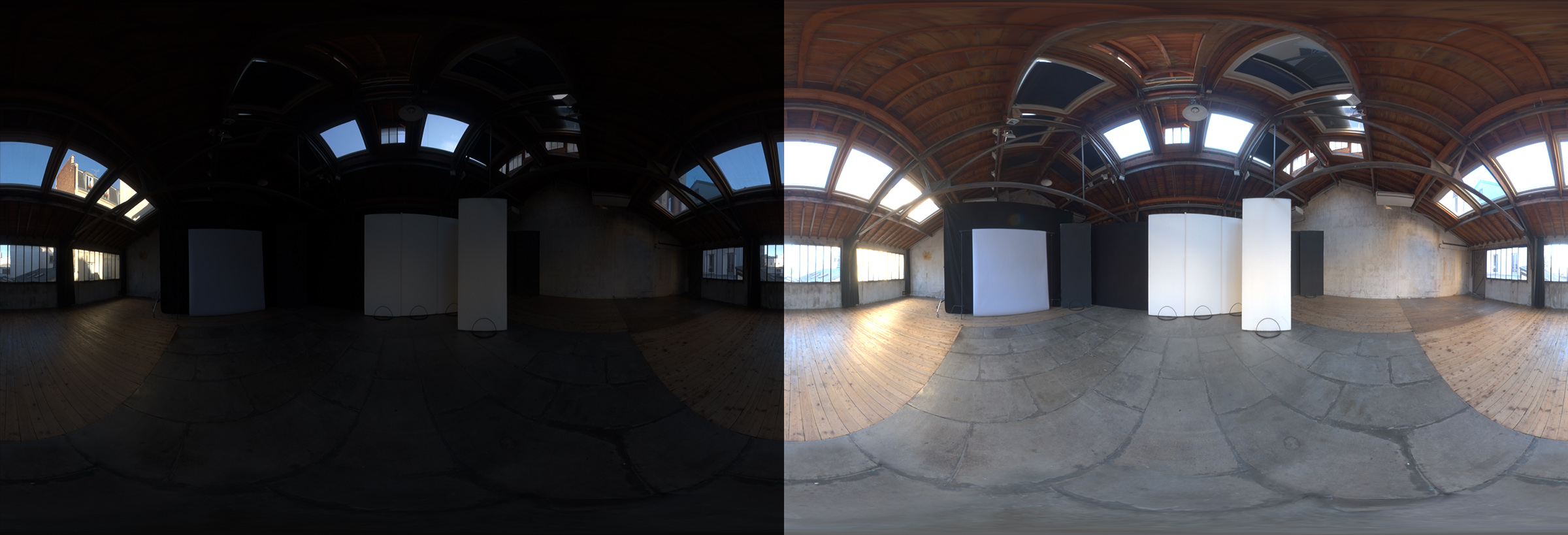
High Dynamic Range Images

As physical illumination in the real world takes both very high and very low values, the total dynamic range can be huge (reaching an order of $10^14$ at the extremes — complete darkness / direct sunlight). Therefore, representing illumination for environment mapping requires formats and numerical representations of extended precision and scale. Specific formats allow for such an extended range of values to be stored, including the TIFF and EXR formats, with EXR being the standard for environment maps. Although directly displaying the entire range of a High Dynamic Range Image (HDRI) is not possible on output devices, without selectively specifying a sub-window of the dynamic range to visualize, the stored information is directly compatible with a physically-based rendering pipeline, which is expected to handle both very large and very low radiance values.

Procedural Sky Models

Sky dome appearance is very important for the rendering of outdoor environments. Correct skylight modeling can often make the difference between a plausible and an unnatural-looking sky. More importantly, certain fields of study and engineering, apart from generating beautiful imagery, require dependable and accurate radiometric illumination. A radiometrically correct model that provides reliable illuminance data is important for application areas like architecture and illumination engineering, where accuracy is important. Unfortunately, physically accurate measurements of this rapidly varying illumination source are difficult to achieve.

One common approach to rendering scenes that are lit by a sky dome is to use environment maps or textures projected on skybox geometry proxies, which use actual photographs of the sky as the source of illumination. These offer high quality lighting for static scenarios but are very expensive to handle in dynamic cases, where we want time-of-day control of the sky and geospatial data for the trajectory of the sun.

As sunlight propagates through a cloudless atmosphere the important interactions are the scattering events in the atmosphere itself, and the reflection of light on the ground. For the purposes of light propagation, the atmosphere can be considered to contain aerosols and air molecules. The interaction of light with these is covered by Lorenz-Mie and Rayleigh scattering theory, respectively. Rayleigh scattering describes the interactions between electromagnetic radiation and particles significantly smaller than the wavelength of the radiation (e.g. visible light). Lorenz-Mie theory provides the framework to predict the contribution of particles of sizes comparable to the wavelength of visible light. Both phenomena can be described and approximated with phase functions that model the probability distribution of the scattering angle of light as it interacts with the medium. Brute-force simulation of a huge number of interactions can create physically-accurate vistas of the sky. However, in the field of computer graphics, approximate solutions are the preferred choice in order to achieve reasonable performance.

Analytical sky models are mathematical sun and sky illumination models, which can be controlled by a small number of intuitive parameters and can be queried by illumination direction to obtain a good approximation of the sky dome luminance with a very small cost. One of the first colored skylight model that is directly useful for rendering purposes was proposed by Perez et al. (Perez, Seals, and Michalsky 1993). It simulated the appearance of the sky due to single scattering only, and ignored inter-reflections between the ground and air particles. Capturing sky dome radiance data for a representative, large number of atmospheric conditions and solar elevations from nature in a reliable manner is a very hard problem. Therefore, a common approach is to acquire reference data via a brute force, physical simulation of the interactions between light and participating media that are relevant to atmospheric light transport. A more convenient model for computer graphics applications was proposed by Preetham et al. (Preetham, Shirley, and Smits 1999). The Preetham model is nowadays implemented in many commercial renderers and included in game engines and ray tracing libraries. Hosek and Wilkie (Hosek and Wilkie 2012) expanded the Preetham model using data generated by an offline volumetric path tracer, taking into account complex atmospheric phenomena. The formula was slightly modified and the values where fitted again. The model produces radiance data that are separately fitted for each color channel, either as spectral values, or CIE XYZ colors.

Sky models are typically parameterized by the sun elevation and azimuth and also controlled by a turbidity factor that defines how intense is the scattering due to the presence of aerosols. These intuitive parameters are then mapped to the internal parameterization of each model in order to compute the sky luminance.

Shadows

Wherever there is light, there are shadows. The presence of shadows is inherent in the light propagation process, due to the obstruction of the light paths by geometry and denser pockets of the transmission medium. Most of the time, light intercepted by a body is also out-scattered, contributing to the global illumination of the environment. However, here we examine the obstruction of light as an isolated phenomenon, from the point of view of the intended receiver. In this sense, shadowing is a visibility determination task, boiling down to determining whether a shaded point is accessible by a particular point on an emissive surface. The resulting loss of radiant energy we call direct shadows. Shadows from direct lighting are generally of higher contrast compared to the general illumination level of the environment, since the energy coming directly from the emitters has not yet been attenuated by scattering and absorption and its loss (obstruction) causes a significant drop to the contributed illumination.

In computer graphics, we simulate shadows in various ways, as a specialized visibility determination task, depending on the implementation of the rendering pipeline (see relevant rendering unit), but their importance transcend aesthetic purposes. It is true that shadows, at least from direct lighting are "expected" in the rendering of a virtual environment in order to look "right". However, why are shadows so important to our perception of the world? How do they help us understand the geometry we are visualizing and our role in the virtual environment?

• Shadows provide clues about the shape and volume of the geometry. The interplay of light on the surface and the resulting occlusions reveal detail, protrusions and crevices, deep recesses and ridges.

• They help us place the objects in the environment, providing clues about relative distances. This is demonstrated in the following figure. The closeness or detachment of an object’s shadow is indicative of its relative distance to its surroundings and its relative scale.

• Shadows enhance depth perception, especially in monocular vision, where the human visual system relies on clues and recognizable configurations to discern the ordering and distances of objects.

• They bolster the sense of light direction and by extent, self orientation.

• The blocking of light enhances the visual detail of the displayed surfaces by enhancing local contrast, making the visual content more interesting and rich.

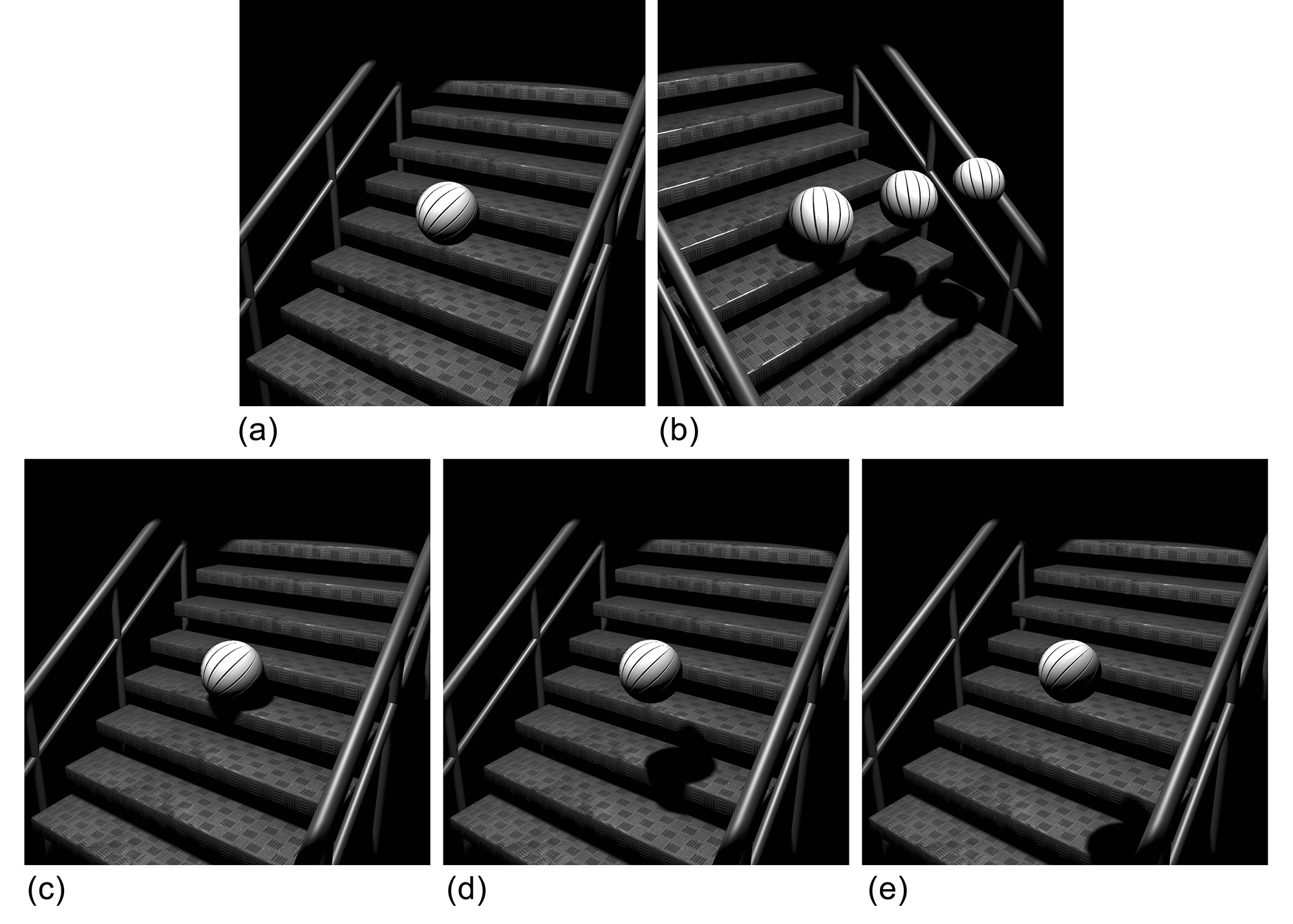
Hard and Soft shadows

The exact shape of the shadow is influenced by the proximity of the light source to the shadow casters, as well as the size of the light emitter. A shadow consists of two zones, the umbra, which is the surface region, where light from any part of a particular light source is completely obstructed, and the penumbra, which is partially lit by the light-emitting source. In order for a surface to be partially in shadow, the light source needs to be of non-negligible volume⁴ compared to the size of the objects. To be more precise, as distance affects the apparent size of objects, the apparent projection of the light emitter on the surface needs to be non-negligible to create a penumbra. The shadows that are caused by non-infinitesimal light sources and have both an umbra and a penumbra are called soft shadows. Hard shadows only consist of an umbra and are caused by punctual light sources, or too small ones to have a perceptible penumbra.

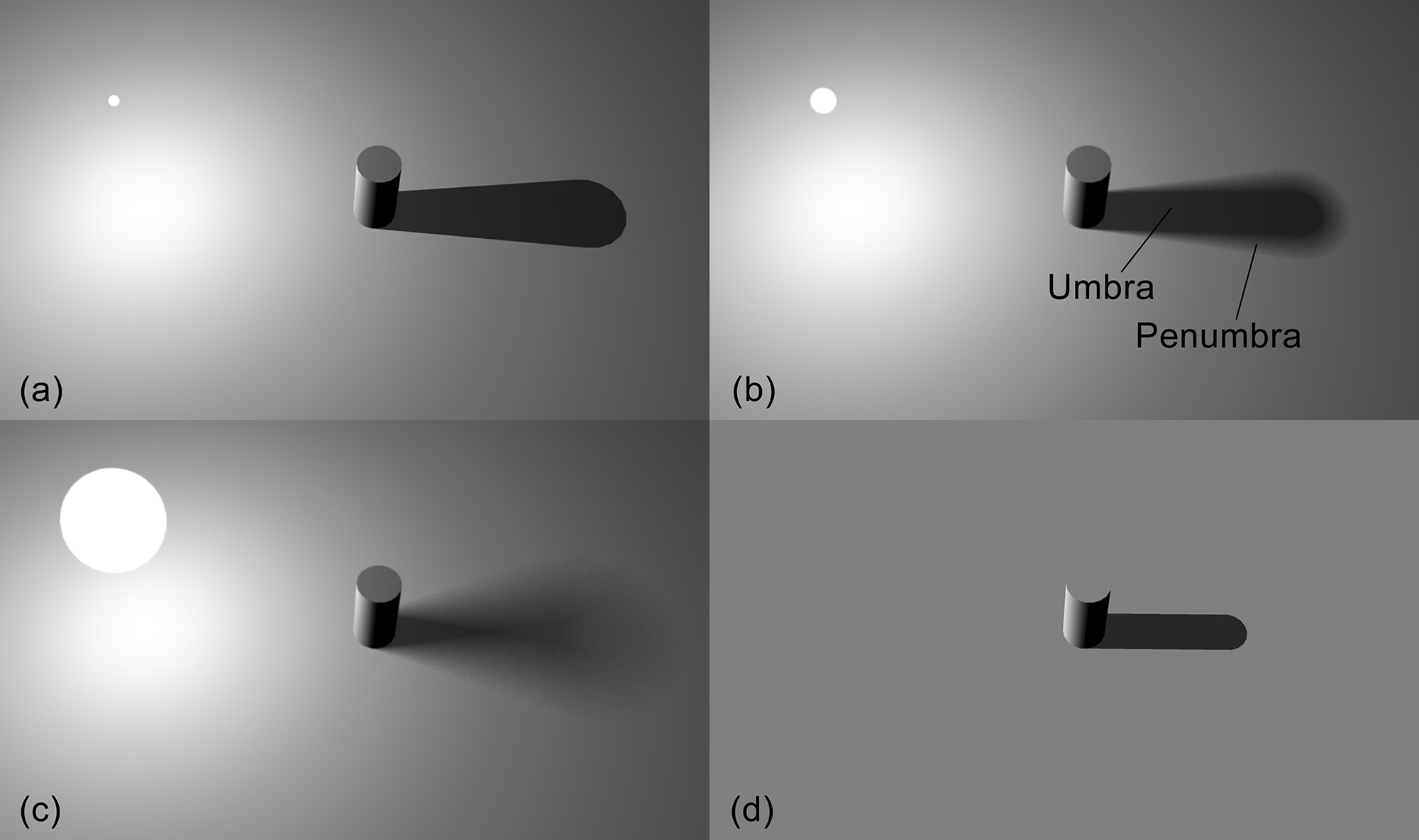
Scattering and indirect shadows

Surfaces not directly lit by a light-emitting surface are not in complete darkness, since light scatters on or through surfaces and indirectly illuminates other parts that do not have a direct access to the provided energy. Visibility determination is obviously important in secondary light bounces, since scattered light is also intercepted by the closest surfaces, causing indirect shadowing on other areas of the scene. If the obstructed light comes from a scattering event, i.e. after the emitted light first scatters on one or more surfaces, we consider the obstruction of light as indirect shadows.

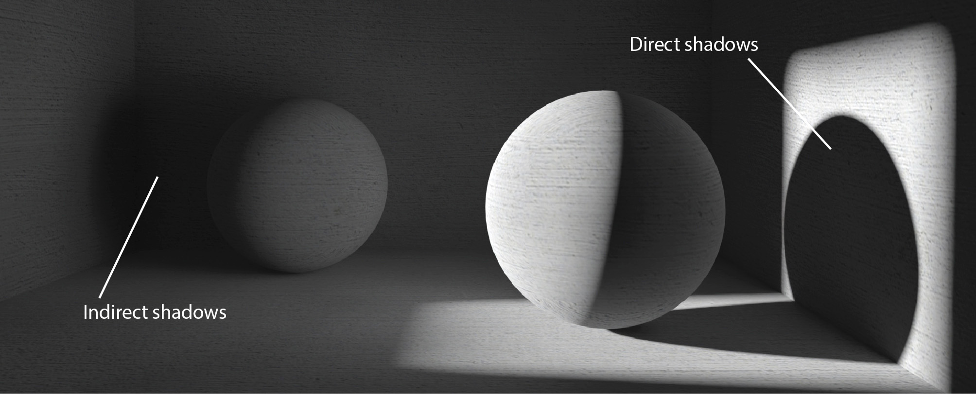
Ambient Occlusion

Ambient occlusion is a physically inspired but not physically based technique that was initially introduced to accentuate geometric features on non-directly lit surfaces during real-time rendering. In the older days of real-time rendering, when the computation and application of indirect lighting was deemed prohibitive, it was popular to use a constant ambient color to represent the average non-directional illumination incident on surfaces. This meant that a flat color was multiplied with the albedo of the surface and direct lighting was added on top of that in an attempt to avoid drawing unlit surfaces black. This invariably caused geometry to look flat and unnatural, however.

A key observation is that, even uniform illumination, cannot illuminate all surfaces equally, since different surface points are exposed in a different manner to light, because other parts of the models and the environment are in the way (Zhukov, Iones, and Kronin 1998). The term ambient occlusion (AO) became popular in the early 2000s, to express how obscured a point is, i.e. how inaccessible it is by uniform, distant lighting. Practical implementations usually compute 1 - AO (ambient "visibility") and still call it ambient occlusion, since this is a term multiplicatively applied to lighting to suppress it, where occlusion is high. It is a normalized term, ranging from 0 (full occlusion) to 1 (full visibility). AO can be precomputed for locations on the geometry per object, either for that object in isolation or within a complete virtual environment, and stored in texture maps or as vertex information (usually the former).

Ambient occlusion is statistically computed and cached by testing the visibility of a location on the geometry in a set of sampled directions on the hemisphere "above" the point, i.e. randomly sampled directions on the normal-aligned hemisphere at the point in question. Typical computations involve casting rays up to a distance $R$ and checking for intersection with any geometry. If an intersection is found, this direction counts as being obstructed, otherwise it is considered open. The query range $R$ can be unbounded or set to a small radius that only considers the blocking of light at the "near field" of the object. A large radius is useful when using AO to suppress lighting coming from a distant spherical environment light, such as a bright sky dome. A small radius is more handy when we precompute AO texture maps for individual objects and then combine them in a single environment, where their mutual occlusion is not known beforehand and only near-field (localized) interference can be pre-calculated.

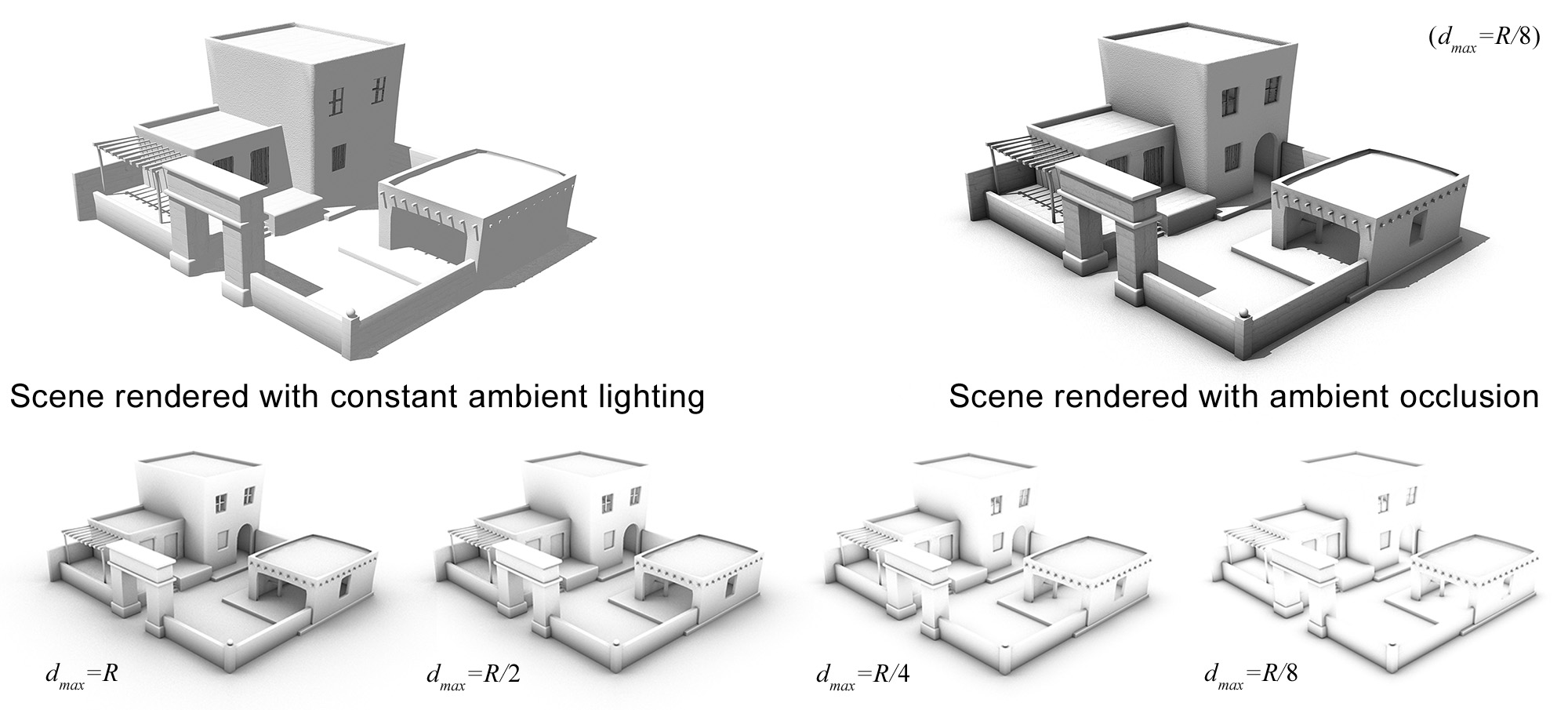
Applying ambient occlusion is rather tricky as it is a non-directional quantity. It only makes sence for attenuating uniformly distributed illumination and in the past yeas it has been erroneously used in many situations, most notably being the attenuation of direct illumination from directional lights and local light sources. In many interactive applications (including but not limited to games) it has been used as a simplified geometry-aware local contrast enhancement method, rather than a method for physically-based lighting. However, despite not being a physically correct illumination approach, it greatly improved the application of a constant ambient illumination level, as can be observed in the following example.

References

---

1. Except for very thin metallic films, which let some light through. These can be modeled in graphics by combining different shading models to achieve the intended effect, or by diminishing the metallicity of a surface.↩︎

2. A texture coordinate assigned to a vertex can be outside the normalized range, to allow for remapping operations to "wrap" the coordinates around, "mirror" them, etc.↩︎

3. Sampling theorem: https://en.wikipedia.org/wiki/Nyquist%E2%80%93Shannon_sampling_theorem↩︎

4. More precisely, the light source’s projection in the direction of illumination on the surface has to be of non-zero area.↩︎