2D and 3D Shape Representation

Coordinate Systems

Both in two- and three-dimensional space (in fact in any $n$-dimensional one) we can establish a set of coordinates to relate a particular point with respect to a reference point and set of axes. We have done this already in 2D image space, where an image coordinate system (ICS) was implied, when enumerating pixels in an image grid from its upper left or lower left corner and measured along a horizontal and vertical direction spanning the image plane.

In order to define the coordinates of every vector, in 2D we use a pair of mutually orthogonal basis vectors $\vec{\mathbf{i}}, \vec{\mathbf{j}}$ and in 3D space we extend this construct with another vector $\vec{\mathbf{k}}$ perpendicular to the first two ones, as shown in the figure below. For an arbitrary vector $\vec{\mathbf{v}}$, its coordinates $(x,y)$ or $(x,y,z)$ represent the dependence of the vector to (or the "similarity" of the vector with) the two or three coordinate frame vectors. The coordinates are essentially the projection of the vector onto $\vec{\mathbf{i}}$, $\vec{\mathbf{j}}$ and $\vec{\mathbf{k}}$.

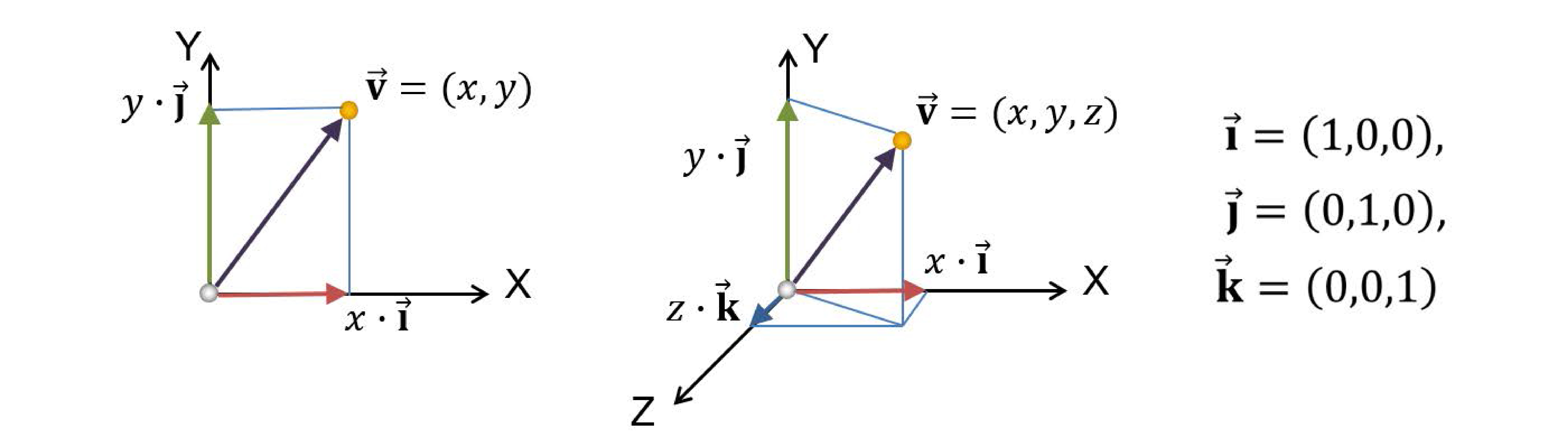
Now, unless we add a reference vector or origin to the coordinate system, against which all other vectors are compared with respect to their coordinates, we cannot define absolute positions in space; consider the axis system as a floating frame in space, where only directions can be established. If we lock this system down by appointing an origin, then we can fully describe points, i.e. vectors starting from the origin and ending at the particular location in space. In the following text we denote points as bold upright letters, e.g. $\mathbf{p}$, although for simplicity we also refer to vectors using the same notation.

Planar Shapes

An aggregation of primitives or elementary drawing shapes, combined with specific rules and manipulation operations to construct meaningful entities constitutes a geometric representation. In two dimensions, these may comprise a drawing, a collection of text glyphs or any other planar set of shapes. The three-dimensional counterpart is a virtual environment or a three-dimensional scene (see also the preliminaries unit). In both cases, the basic building blocks for modeling, representing and recognizing the shapes are primitives, which are essentially mathematical representations of simple shapes such as lines, curves, points in space, mathematical solids or functions.

To synthesize images from two-dimensional drawings, think of a canvas, where text, line drawings and other shapes are arranged in specific locations by manipulating them on a plane or directly drawing curves on the canvas. Everything is expressed in the reference frame of the canvas, possibly in real-world units. We then need to display this mathematically defined document in a window, e.g. on our favorite word processing or document publishing application. What we define is a virtual window in the possibly infinite space of the document canvas. We then ‘capture’ (render) the contents of the window into an image buffer by converting the transformed mathematical representations visible within the window to pixel intensities at specific sample locations.

We will now go over some of the most commonly used shape primitives for planar shapes to define their properties and see how they can form collections to synthesize more elaborate entities.

Line Segments

The simplest form of a two-dimensional shape that we can define and represent is a line segment or linear edge (if we refer to a boundary of a filled shape). It is defined by its two endpoints $\mathbf{p}_0$ and $\mathbf{p}_1$: $\mathbf{p}_0\mathbf{p}_1$ and can be oriented in the sense that the particular ordering of its endpoints defines a vector indicating the forward direction on the line passing through them. Mathematically, two specific points on the plane define a singular mathematical line on the plane:

$$\label{eq_line1} \mathbf{p} = \mathbf{p}_0 + t (\mathbf{p}_1-\mathbf{p}_0),$$

where $t$ is a scalar. The above equation is the parametric line equation, i.e. defines a new point on the two-dimensional plane constrained on the line as a combination of the two known locations $\mathbf{p}_1, \mathbf{p}_0$. The free parameter $t$ is allowed to take arbitrary values, each time generating a new point on the line. Negative values of $t$ produce points ‘before’ $\mathbf{p}_0$ (with respect to the ordering of points on the line), whereas values of $t>1$ define points beyond $\mathbf{p}_1$. In this respect, $t$ acts as a linear interpolation parameter between the two points, i.e. produces points linearly dependent on the two fixed locations.

An alternative (yet equivalent) form of the equation of a straight line is defined by:

$$\label{eq_line2} ax + by + c = 0,$$

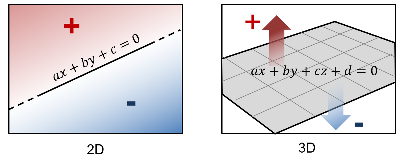
where $a, b$ are not both 0. The coefficients a and b in the general equation are the components of vector $\mathbf{n} = (a, b)$ perpendicular to the line. We will extensively use the notion of a vector "perpendicular to" a primitive defining a boundary, since it defines its orientation precisely. When this orientation vector is also unit-sized, i.e. its length is 1, we call this, the normal vector.

The line equation splits the plane into two half-planes or half-spaces as is the general term. Calculating the result of the formula $ax + by + c$ for any point on the plane $\mathbf{p}=(x,y)$, we can test whether $\mathbf{p}$ lies on the boundary (the line itself), the left or the right half-plane. If the result is $0$, the point lies on the (infinite) line. If it is greater than zero $\mathbf{p}$ lies on the ‘left’ half-plane, where the normal vector points at, otherwise, it lies on the right half-plane. We will discuss later that such a test is used for determining containment of a point in a convex region.

The notion of the parametric line equation is trivial to extent to multiple dimensions, by simply defining the two vertices in a higher-dimensional space, e.g. the three-dimensional Euclidean space. However, whereas the 2D line splits the plane in two half-spaces, the same does not hold in higher dimensions. In general, for a $k$-dimensional space, we require an unbounded manifold of $k-1$ dimensions to divide the space into two subspaces. For example, in 3D space a surface such as an infinite plane or a sphere cuts the space in two open subspaces or one open and one compact (the interior of the sphere), respectively.

Polylines and Triangles

Consider now $n$ linear segments on after the other, each sharing a common vertex with the previous one: $\mathbf{p}_0\mathbf{p}_1...\mathbf{p}_n$. These segments form a polyline (polygonal line), or more formally, a piece-wise linear curve. If the $n$-th vertex is connected to or coincides with the first vertex ($\mathbf{p}_0$), then the polyline forms a closed boundary.

Similar to the fact that in general points on a two-dimensional polyline do not all lie on a straight line, the vertices of a polyline in the three-dimensional space are not necessarily on the same plane. The only polygonal shape that guarantees this is the triangle.

Furthermore, the triangle is a minimal convex shape, with the important property for computer graphics and shape analysis that for a triangle with vertices $\mathbf{p}_0\mathbf{p}_1\mathbf{p}_2$, any linear combination of the form $\mathbf{p}=a_0\mathbf{p}_0 + a_1\mathbf{p}_1 + a_2\mathbf{p}_2$ with $0\leq a_i \leq 1$ and $a_0 + a_1 + a_2 = 1$ is guaranteed to lie on the triangle. This property is very frequently used to identify interior points to a triangle and interpolate values at them from the three vertices, when sampling and filling the interior of triangulated shapes.

Filled Regions

Given a closed boundary of a manifold, e.g. a circle on the plane, we can always define an interior region for it. For many well-defined (convex) shapes such as ellipses, triangles, rectangles etc., determining whether a point lies on the interior of the boundary is trivial. As we will see next, more complex boundaries can be approximated by polylines and then triangulated.

Remark: The interior of any closed non-self-intersecting polyline on the plane can be represented by a set of triangles.

A triangle can be easily sampled in order to be colorized with a fill color, gradient or pattern, by determining image-space samples in its interior and computing a color for them.

Bézier Curves

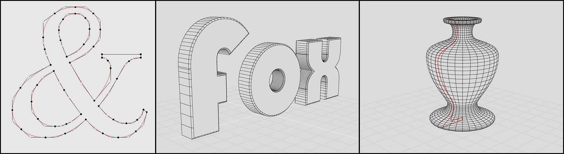
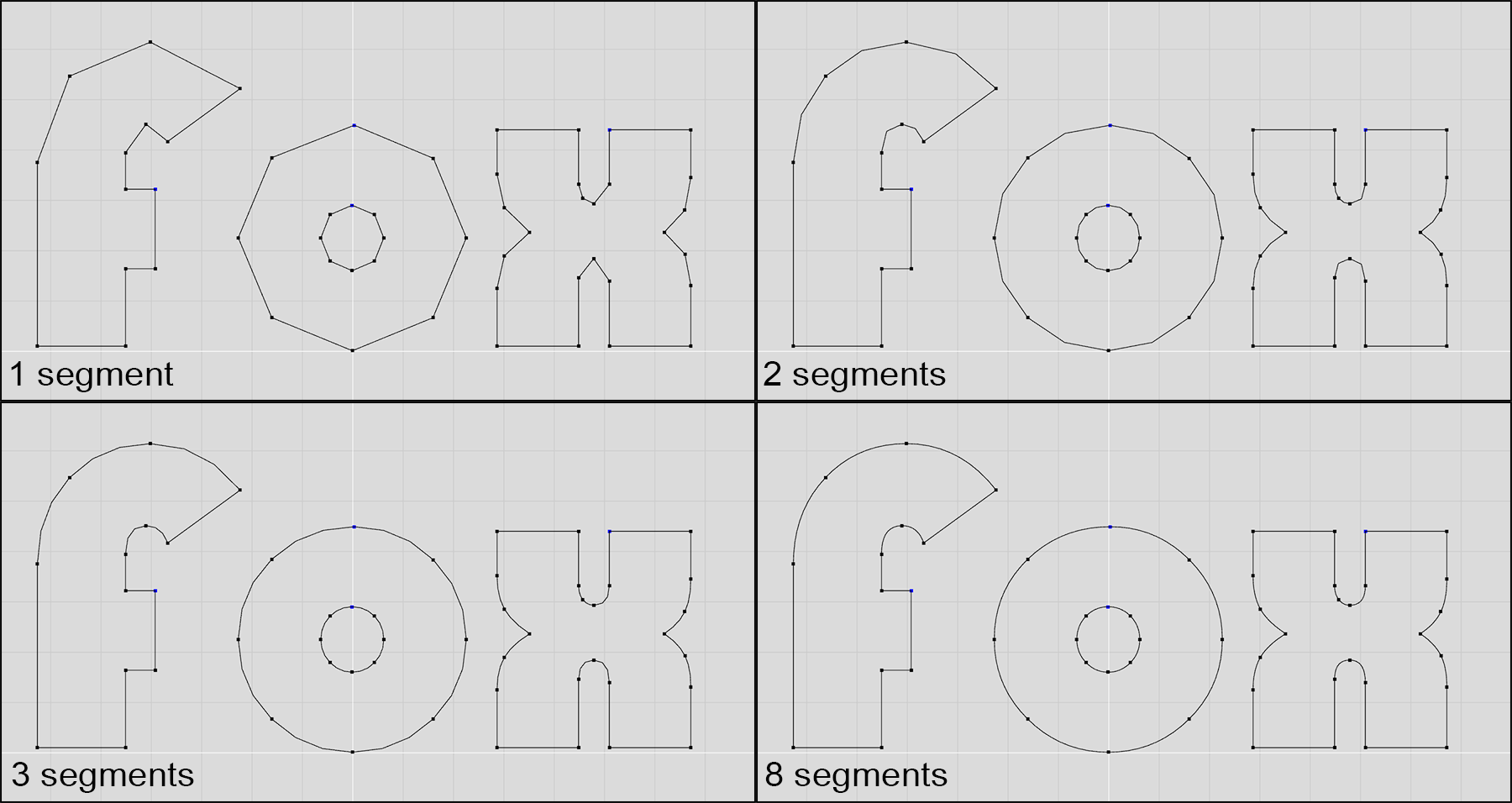
Linear segments are useful for drawing and representing clean, straight edges on the boundaries of shapes. However, it is often desired that a boundary should be curved. In mathematics, curves cannot be represented exactly using linear segments, and can only be approximated by polylines, resulting in jugged edges. Curves are typically represented by non-linear formulas, such as polynomials. A particular family of parametric polynomial functions, that are tremendously useful in shape representation are the Bézier curves. The term "parametric" again represents the fact that the curve evolves on the plane as a function of a parameter $t$ that "runs" over the trajectory of the curve to define every possible point on it, similar to the parameter of the line equation above.

An important characteristic of the Bézier curves, is their degree. All polynomial functions are characterized by their degree, which is the largest exponent used in their formula. The higher the degree, the smoother the curve and the larger the number of the supporting, or control points becomes. The latter means that in order to be able to define a smooth Bézier curve, we need to define more than its end points. In the case of a linear segment, which can be regarded as a Bézier curve of degree 1, by the way, two points on the plane fully described the unique line passing through them. As we add more degrees of freedom however, we need more information (points on the plane here) to "control" and restrict the trajectory of the curve on a single shape. In the general case, an $n$-th degree Bézier curve $\mathbf{P}^n(t)$ may be constructed given $(n+1)$ control points $\mathbf{p}_0, \mathbf{p}_1, \ldots, \mathbf{p}_n$.

The exact formula of the Bézier curve is outside the scope of this text, but suffice to say the definition of the curve is an elegant recursive linear interpolation, which uses the polyline connecting the control points as a "cage" to bound and control the shape of the curve. For more formal definition of Bézier curves and other parametric curves and surfaces, please see (Theoharis et al. 2008).

Why are Bézier curves important? Any curved boundary on the plane or trajectory in 3D space can be defined as a collection of connected Bézier curve segments, providing a powerful tool for the accurate representation of shapes such as text and other vector graphics. Curves are an important design tool, not only for 2D graphics, but also for defining and extruding curves to form surfaces, creating surfaces of revolution out of a curved profile or determining three-dimensional trajectories for animated entities, where the $t$ parameter is interpreted as the time variable.

In rendering, for simplicity and efficiency it is often helpful to operate on a single type of primitives. Linear forms, such as line segments, triangles and other planar polygons are usually preferred, as they can approximate other forms at an arbitrary level of precision, trading accuracy for uniformity in terms of processing, rendering algorithms and hardware implementations. Therefore, it is often the case that a parametric curve is sampled to create intermediate points on a curved segment, which are then joined to form a polyline that approximates the curve function. The more steps one takes, the better the polyline approximates the curve. Sometimes, the number of samples is determined adaptively, based on the approximation error. In other implementations, the sampling rate is dynamically determined according to the desired precision, which in turn is determined by factors such as zoom level and image resolution.

Common Formats

There are numerous formats for storing vectorized information, primarily due to the fact that there is a long history of computer aided design (CAD) applications that have established a number of widely accepted formats for design storage. Another reason is the necessity to describe glyphs and shapes for reproduction on printing and plotting devices, as well as computer-controlled milling machines and cutters. In the last decades, with the prevalence of web-based graphics and the need to exchange digital documents and high-fidelity yet low-bandwidth visual information, many old formats have been extensively enriched and new ones have emerged.

The most commonly adopted vector graphics format is the Portable Document Format (PDF) developed in the 1990s by Adobe Systems. Aside from vector primitives, gradients and fill patterns, it supports a complex encapsulation mechanism for including raster information, embedded fonts etc. in the same container. PDF supports structured information, with hyperlinks and indexing and is designed for the representation of entire documents, but is very frequently used for single drawings and designs.

A simpler specification for defining, storing and displaying shapes is the Scalable Vector Graphics (SVG) format. This XML-based shape description language was designed for the representation of vectorized information for the web and was introduced in 1999. It is since then extensively used for the display of shapes in web graphics.

The AutoCAD Drawing Interchange Format (DXF) established and updated by Autodesk is one of the oldest vector graphics formats and was designed for the importing and exporting of CAD drawings to and from various CAD programs and their interoperability with the company’s own established CAD ecosystem. Despite its focus on mechanical and architectural design, due to its generality, it has been extensively used for the representation of generic drawings and has been frequently used in the past for archaeological documentation.

Three-dimensional Data

Three-dimensional information varies both in form and representation, depending on the application domain and the technology the data are related to, generated by or acquired from. We will examine next the most basic and commonly used forms of 3D data representations and formats.

Three-dimensional Coordinate Systems

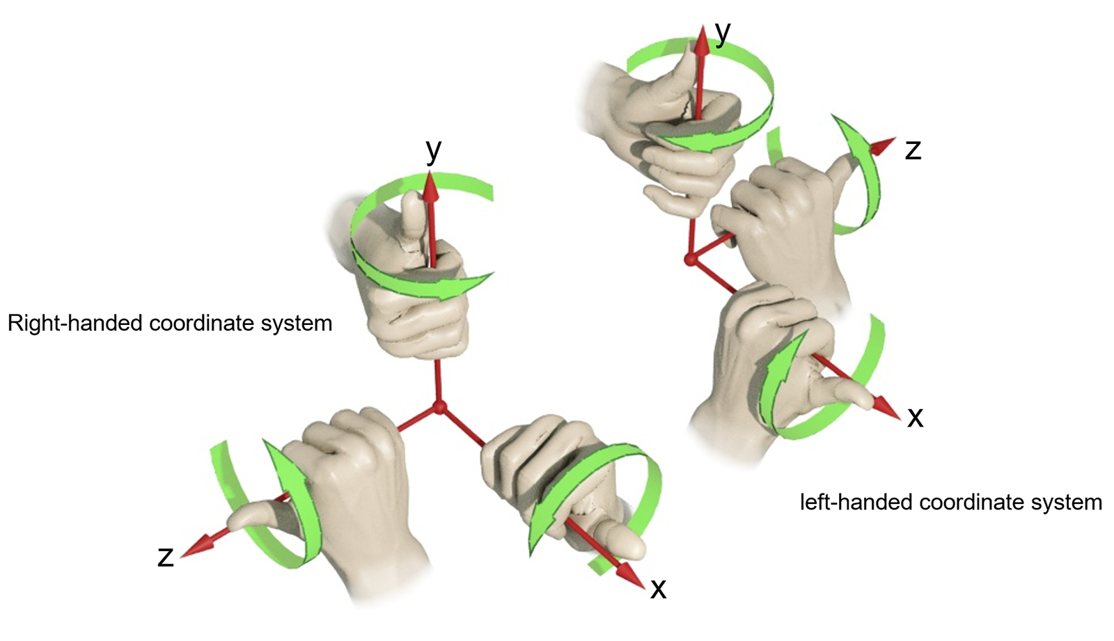
Three-dimensional coordinate systems augment the planar Euclidean space with a third, "depth" dimension. We can define a "right-handed" coordinate system, where the Z (depth) axis points out of the plane towards the observer. Conversely, we can define a "left-handed" coordinate system, in which the Z axis points forward. In most applications dealing with 3D data, the right-handed coordinate system is used. The name comes from the fact that in such a coordinate system, the positive angles for defining rotations can be determined by the rule of the thumb: when the thumb is placed along the positive axis the rotation is performed around, the curl of the hand indicates the positive turn direction. This is illustrated in the following figure.

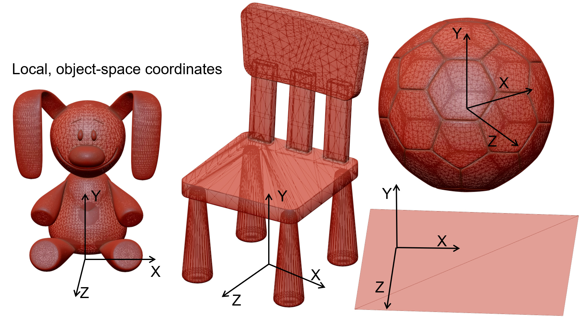
When working in three-dimensional space, there is no "objective" reference frame to measure distances and coordinates from. For example, if we capture the shape of an object with a 3D digitization device, the system establishes its own coordinate system, typically centered at one of its sensors. The recorded coordinates are then exported to a file. In the same spirit, if we create a model of an object using some modeling software, we arbitrarily establish an origin for it and describe the surface’s coordinates according to it. This point of reference (the origin), along with the corresponding primary axes $\vec{\mathbf{i}}$, $\vec{\mathbf{j}}$, $\vec{\mathbf{k}}$ we used comprise the Object Coordinate System (OCS) of the object, in the sense that they represent the shape in isolation, with no regard for other shapes or a global arrangement of the object in a virtual set.

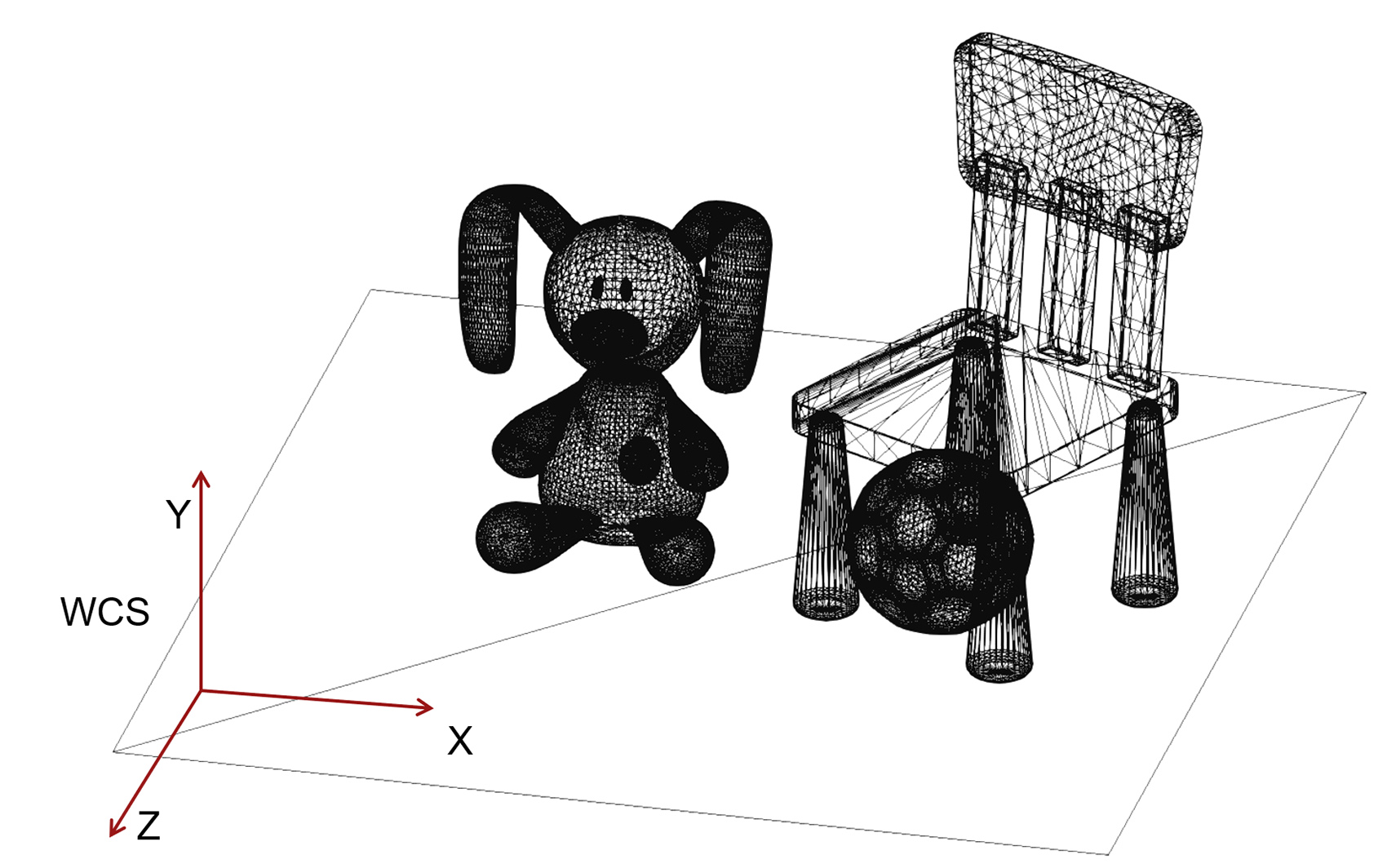
In many situations, predominately when compiling a virtual environment out of many created or captured 3D models, the loaded 3D models must be arranged in relative poses to each other that will result in the vertices of these models having different coordinates than the originally recorded ones in the files that we loaded. To achieve this, we typically apply a geometric transformation (see next) to the coordinates of the models to change them relative to a common (global) coordinate system that is shared by all the objects in the same virtual environment. This coordinate system is referred to as the World Coordinate System (WCS) as it represents a global (or "world"-wide) reference frame for all the geometry present in the environment.

In the example of the above figure, the 4 models have their own local reference system in which the coordinates of the surfaces have been defined during model creation. If load without any modification, $(0,0,0)$ is also assumed to be the overall coordinate system of the application, i.e. the WCS, which will coincide with the OCS of each model. However, their surfaces will overlap in space, defining no meaningful spatial arrangement. In order to be able to visualize them properly and set up a virtual environment, we need to move them apart so that they do not overlap and form the intended scene. This relative movement that we apply to each object, the geometric transformation, is one of the fundamental geometric operations we perform on geometric entities. It changes the coordinates of the OCS and those of the entire 3D model that is dependent on the reference system, so that both the model’s OCS does not coincide with the WCS any more. Each object has now two different coordinate representations: one with respect to its local reference frame (OCS) and one with respect to the global reference system (WCS).

Let us now add a virtual camera to this set, i.e. an observation point in space looking towards a particular direction (the virtual "eye"). The camera defines its own reference frame, the Eye Coordinate System (ECS) and at any given time it can represent the viewport of the user into the 3D virtual world. Any coordinates of vertices expressed with respect to it are "ego-centric", in the sense that they express where shapes appear from the user’s point of view.

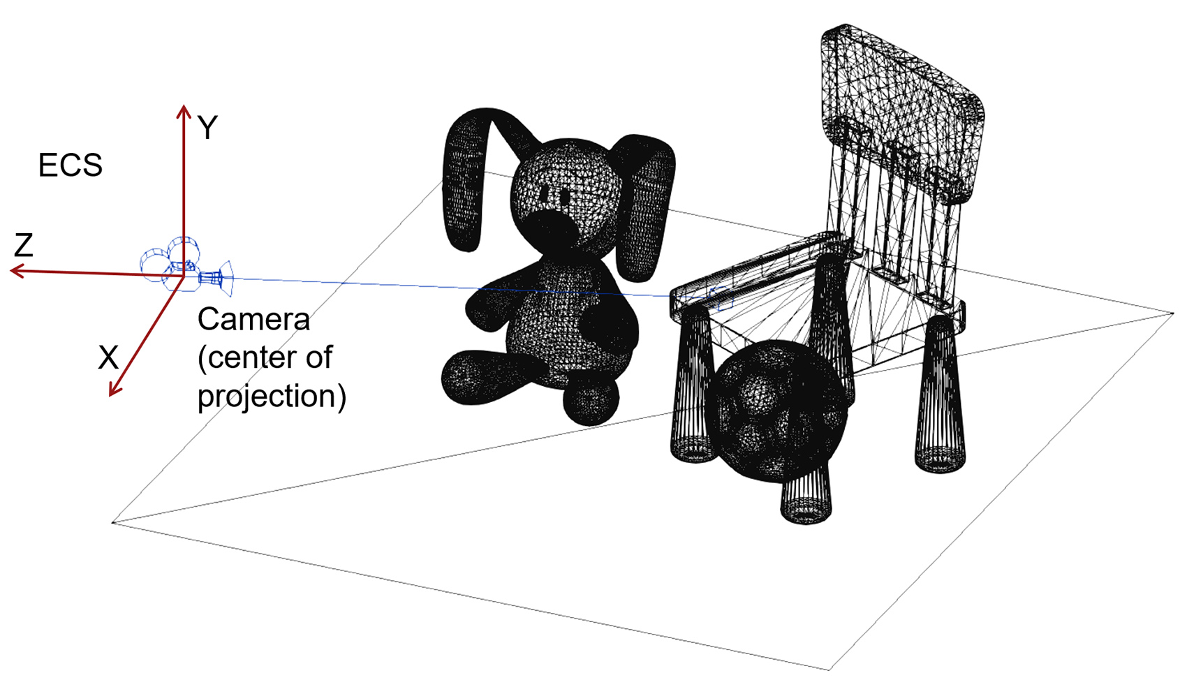
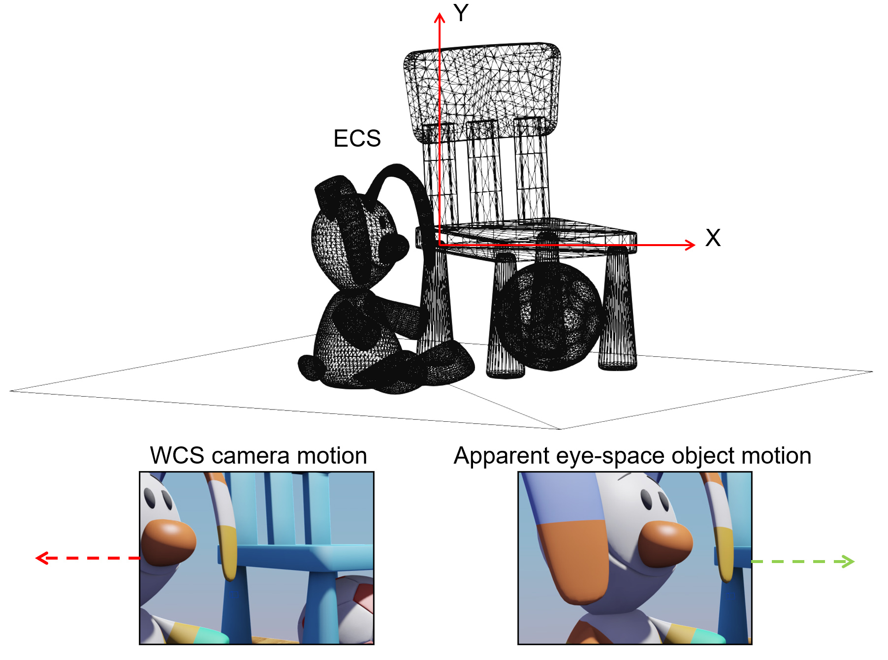
If we move the camera right, i.e. along the X axis of the ECS coordinate system, in our "eyes", the world appears to be moving to the left, as the relative position of the the ECS and WCS change. This is a characteristic duality between transforming the objects and transforming the coordinate system: applying a forward geometric transformation to the coordinate system (here moving the camera to the right) and leaving the shapes stationary has the same effect as inversely transforming the shapes (here moving them to the left) and keeping the coordinate system still.

In the rasterization pipeline ², objects need to be projected on the image plane to acquire their "footprint" on the virtual image sensor plane. The projection can be perspective or parallel, an idealized telephoto view of the world with infinite focal length (see more in the viewing and projection section). After projection, and particularly in the case of perspective projection, Coordinates do not retain any linear spatial relation and become perspectively warped. The post-projective space is also normalized in the case of rasterization for computational efficiency and numerical stability (Normalized Device Coordinates).

Finally, all coordinates must be expressed in terms of viewport coordinates, in pixel units so that they are in line with the raster density of the formed image. Using these final image-space coordinates we can perform the sampling of the primitives in the rasterization pipeline and fill the image buffer with the shaded values for these samples:

The overall sequence of transformations from local object space of the individual constituent parts of a scene, to the final image domain is presented in the following figure. Bear in mind that only the rasterization pipeline needs to perform all transformation stages, as other rendering pipelines may only need to transform objects up to the WCS (e.g. ray tracing systems).

2.5D Data

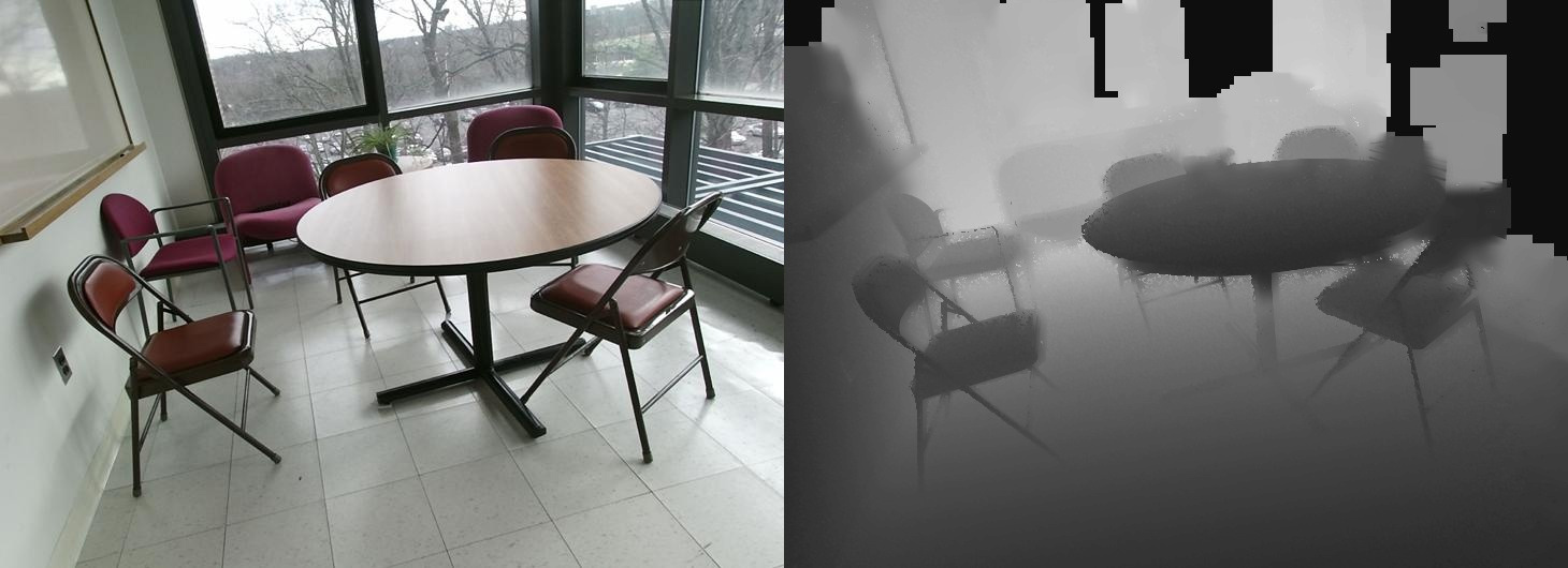
In the simplest form, three-dimensional information may represent a third coordinate dependent on the coordinates on a two-dimensional field: $z=f(x,y)$. This is commonly referred to as a height field, a depth map, or a range map because it maps a two-dimensional coordinate pair to a depth/distance (z) value. Depth maps are often the product of a rendering process, which produces them as a means for resolving which surfaces are visible (see hidden surface elimination in the preliminaries) and constitute internal information to the renderer. However, digitization processes, such as time-of-flight laser scanning, generate such information, which is then used to extract a mesh; multiple range maps (partial scans) are stitched together to form a full 3D model. Given the direct function-like association of a 2D coordinate with a $z$ value, a digitized signal of that form is merely a grey-scale image and is commonly stored as such. This form of three-dimensional representation is also frequently referred to as 2.5D instead of 3D, due to the fact that it cannot describe arbitrary 3D surface coordinates, but rather only $z$ as a function of $(x,y)$.

Point Clouds

The most basic unstructured three-dimensional information that is captured, stored and used for visualization and analysis is an unorganized set of 3D points. Typically, such a point cloud is the result of a digitization process, where the individual members of the point set are samples taken on the surface of a physical object. We call this information a "cloud" to emphasize the fact that the individual members of the set are not connected by some implied or explicitly given structure. This is in contrast to vertices defined as part of a surface modeling process, where connectivity is provided from the beginning, during the formation of the object’s structure. The same holds for certain specific digitization modalities that although result in a set of point samples, these have an implied structure, e.g. they correspond to a range map (see 2.5D data), where samples are arranged on a grid.

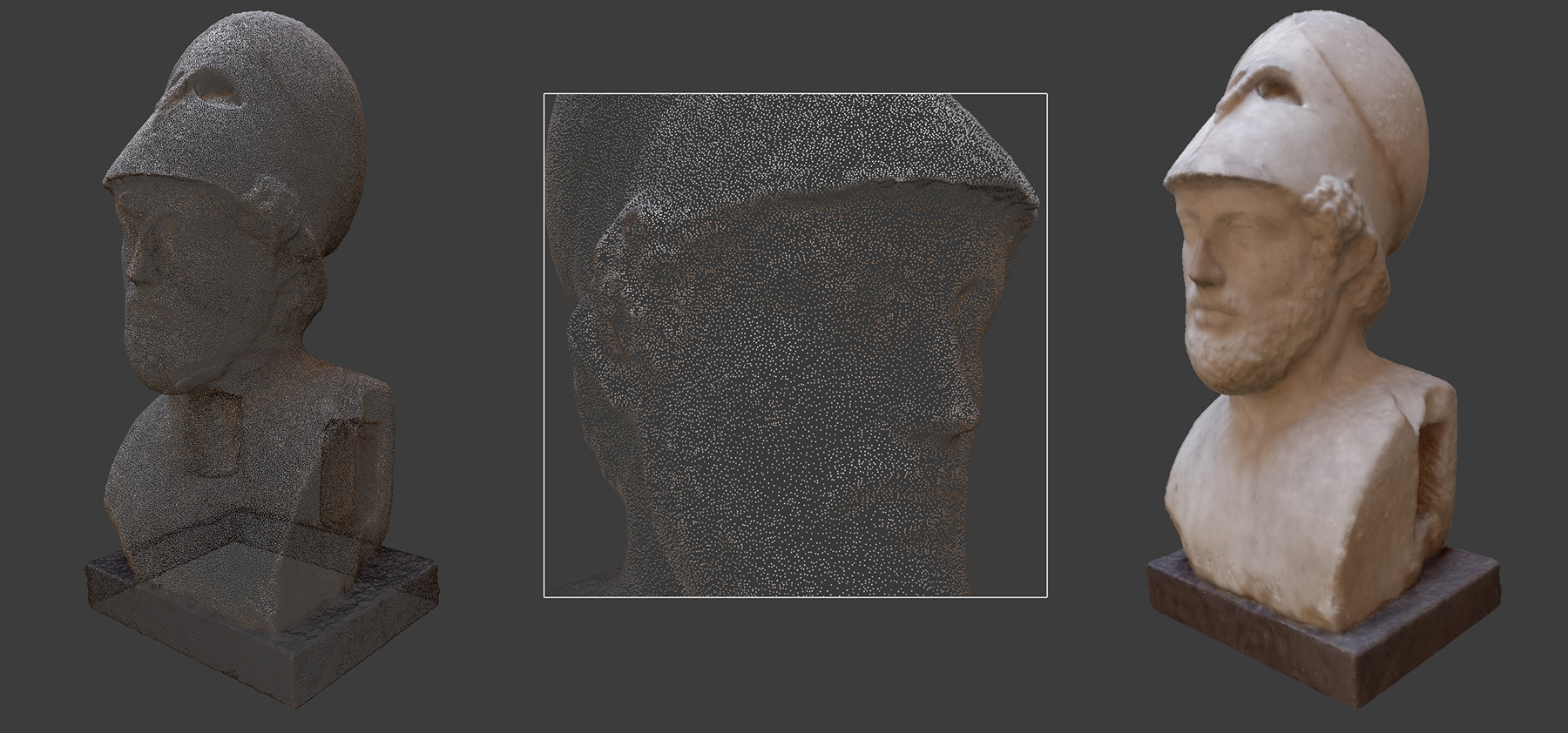
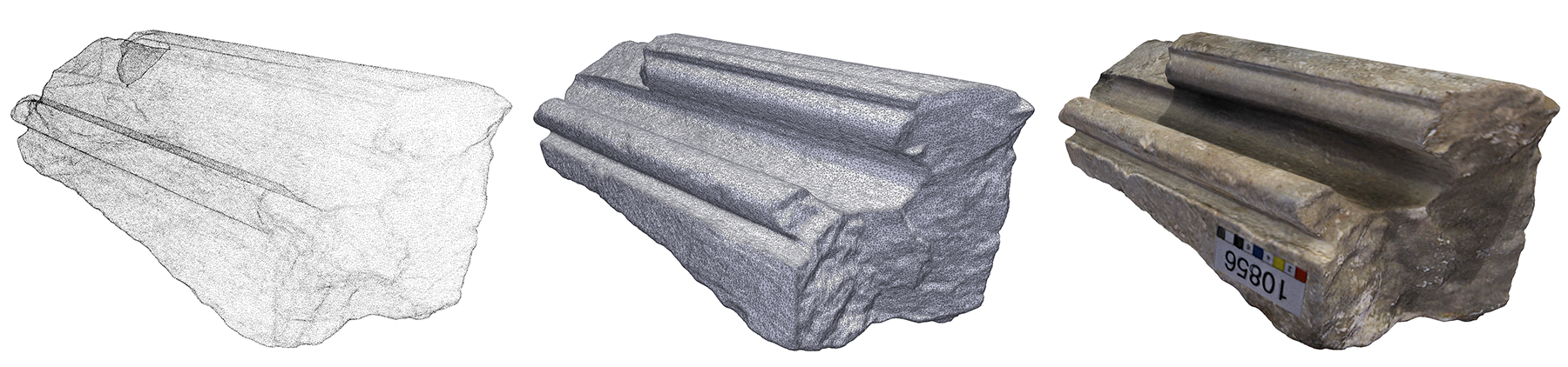
The minimum information stored for each point in a point cloud is the set of Cartesian coordinates of the point, expressed with respect to an OCS. However, additional information may be available per sample, such as albedo or reflectance, calculated surface normals, etc. For examle, the point cloud in the following figure includes position, normal vector and captured albedo per sample (9 scalar values).

The point cloud itself, being a set of discrete, disjoint samples, is not ideally suited for visualization or fabrication purposes, although for many shape analysis algorithms this information alone suffices. In a strict sense, a point cloud, no matter how dense, contains no topological information about how a surface passes through the samples. The given points in space may be interconnected in arbitrary ways to form a surface. However, if a point set is sufficiently dense, the closest points are more likely to be also neighbors in a continuous surface passing through the point cloud. If a raw point cloud is the only information available, meshing algorithms can be used to estimate a surface that wraps over or approximately passes through the given points, often rejecting outliers and filling holes. Please note that such a process often introduces errors and may over-smooth surface details.

Point clouds consisting of many tens of millions of point samples may be hard to interactively visualize as surface models, even in modern real-time rendering architectures. Directly displaying a single point sample on screen is cheaper than also interpolating and displaying pixel values for the surface triangles that connect those points. Therefore, for very large scans, visualization software often uses point-based rendering techniques, that rely on the sheer density of the data set to dispense with the surfacing and respective display of a triangulated mesh. Very often, point-based rendering is combined with normal surface rendering via blending so that distant geometry is visualized as points, while zoomed in parts are displayed as triangulated meshes to avoid seeing through the gaps between adjacent samples.

Surface Meshes

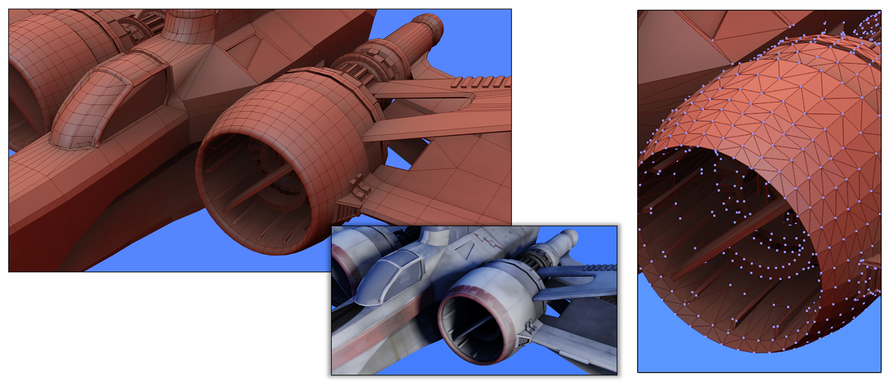
. Given a set of vertices representing samples on a surface, the simplest way to approximate the original geometry is to link the vertices together, forming triangles, as shown in the following figure (right). The triangle is the smallest and simplest polygon and has the very important property that it is always convex. This property greatly simplifies drawing triangles on a computer display by generating pixel-aligned samples in their interior, during rasterization. It also facilitates point containment and line intersection tests for shape processing, manipulation and display. The three vertices of a triangle are always coplanar (by definition) and therefore computing the surface orientation passing through the three vertices is trivial.

Parametric Surfaces

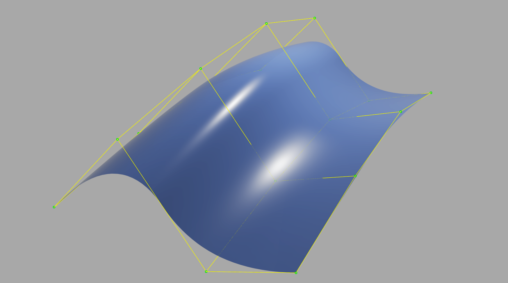
When surfaces are modeled by hand instead of being digitized from real objects, it is often convenient for the artist to work on mathematical representations that allow higher level of control than modifying individual vertices and more accurate definition of smooth surfaces. For this reason, parametric surfaces, an extension of the parametric curves, are frequently the primitives of choice. Bézier , B-spline or NURBS (non-uniform rational B-spline) patches are formed in a similar manner as their 2D cousins, by defining control points (here in space, instead of on the plane). Parametric surfaces allow the modeling of surfaces of arbitrary smoothness. One can always sample a parametric surface at a desired density (can also be variable), to go from parametric surface to point cloud, and finally to a triangulated mesh.

Volumetric representations

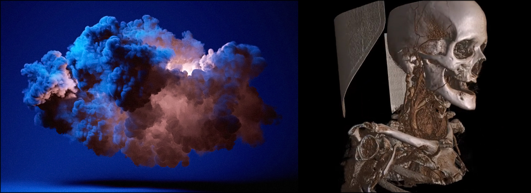
Imaging technology that can capture volume density instead of boundary surface information, such as computed tomography (CT) and magnetic resonance imaging (MRI) scans, results in 3D samples not on 2D surfaces embedded in space, but rather representing a volume contained in a region. Due to the acquisition approach used, these data are typically obtained as computationally reconstructed images that represent slices of the scan volume. Each slice includes a mass density estimation of the medium at that position in space ($x,y$ on the image slice, $z$ being the slice offset). By stacking the individual images, we can treat the resulting layered data as a three-dimensional volume. Traditionally, these slices were individually inspected, but modern 3D graphics allow the real-time visualization of entire volume sets, represented as three-dimensional grids of voxels (volume elements), each voxel storing a density sample. To visualize the density volume, typically density values near a user-provided threshold are retained and colorized, while the remaining voxels are switched off. The retained voxels are then often converted to a surface representation and displayed as usual. In other cases, virtual rays from the camera position are cast, penetrating the volumetric grid and computing illumination on samples of the density volume (volume rendering).

Volumetric representations are important in computer graphics and simulation, beyond the domain of imaging, as they help represent fuzzy data and low-density media that scatter light with low absorption, such as vapor. 3D volume visualization is also very important in physics simulation.

Implicit representations

One way to represent a surface is to consider the boundary of a three-dimensional function $f:\mathbb{R}^3\rightarrow\mathbb{R}$) formed by all the points in space for which the function results in a specific constant value, $f(x,y,z)=d$. This boundary is called a level set. Typically, the entire three-dimensional field of different function values constitutes a signed distance field, with values greater than zero "outside" the isosurface corresponding to the level set of $f(x,y,z) = 0$ and less than zero "inside" the isosurface, representing "negative distances", i.e. offsets from the boundary surface towards the interior of the surface.

A branch of computer graphics addresses the problem of computing and representing fuzzy volumetric information that encodes the spatial distribution of recorded illumination as seen from a number of different viewing angles, in order to be able to reconstruct the represented space from an alternative, new point of view. This task, novel view synthesis, although it uses to some extent algorithms exploited in shape from motion photogrammetry, does not result in a reconstruction of the visible surfaces, but rather an implicit representation of the lighting of the visible space. This implicit radiance field representation is computed by training a hidden representation model over the set of input images, so that the volumetric representation minimizes the distance from the original images when re-evaluated back to form the radiance attended from these specific views. The radiance field is in essence a 5D field that represents the color value of light traveling towards a position $(x,y,z)$ from a direction expressed in polar coordinates $(\phi,\theta)$.

The first significant representative approach of this type of implicit representation is Neural Radiance Fields — NeRFs (Mildenhall et al. 2020), which represents the radiance field as a neural network trained so that during inference, virtual rays traversing the recorded space, can probe the reported volume occupancy and radiance to render the an image similar to conventional volume rendering.

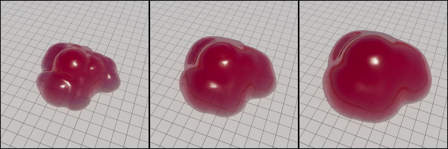
An alternative and highly successful implicit volume representation for novel view synthesis is 3D Gaussian Splats — 3DGS (Kerbl et al. 2023). The method generates and optimizes the parameters of a large number of three-dimensional Gaussian distributions representing the occupancy of space along with directional radiance information. The 3D Gaussians are projected on screen during run time and blended to form the image from the intended view point. 3D Gaussians fully take advantage of the rasterization graphics hardware to generate arbitrary novel views in real time. 3DGS data tend to be massive yet intuitive to process and optimize.

Both NeRFs and 3DGS are becoming a viable alternative to 3D meshes for recording and representing real physical spaces and artefacts.

Shared Vertex Data and Indexing

It is more often than not the case that mesh polygons share vertices, which not only lie on the same 3D coordinates, but also have common secondary attributes, such as vertex color or vertex normal vector. Taking advantage of this fact helps create more compact representations for the data involved in the processing and display of these polygonal meshes.

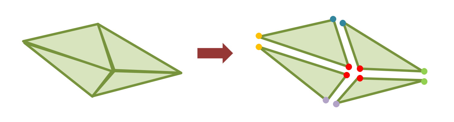
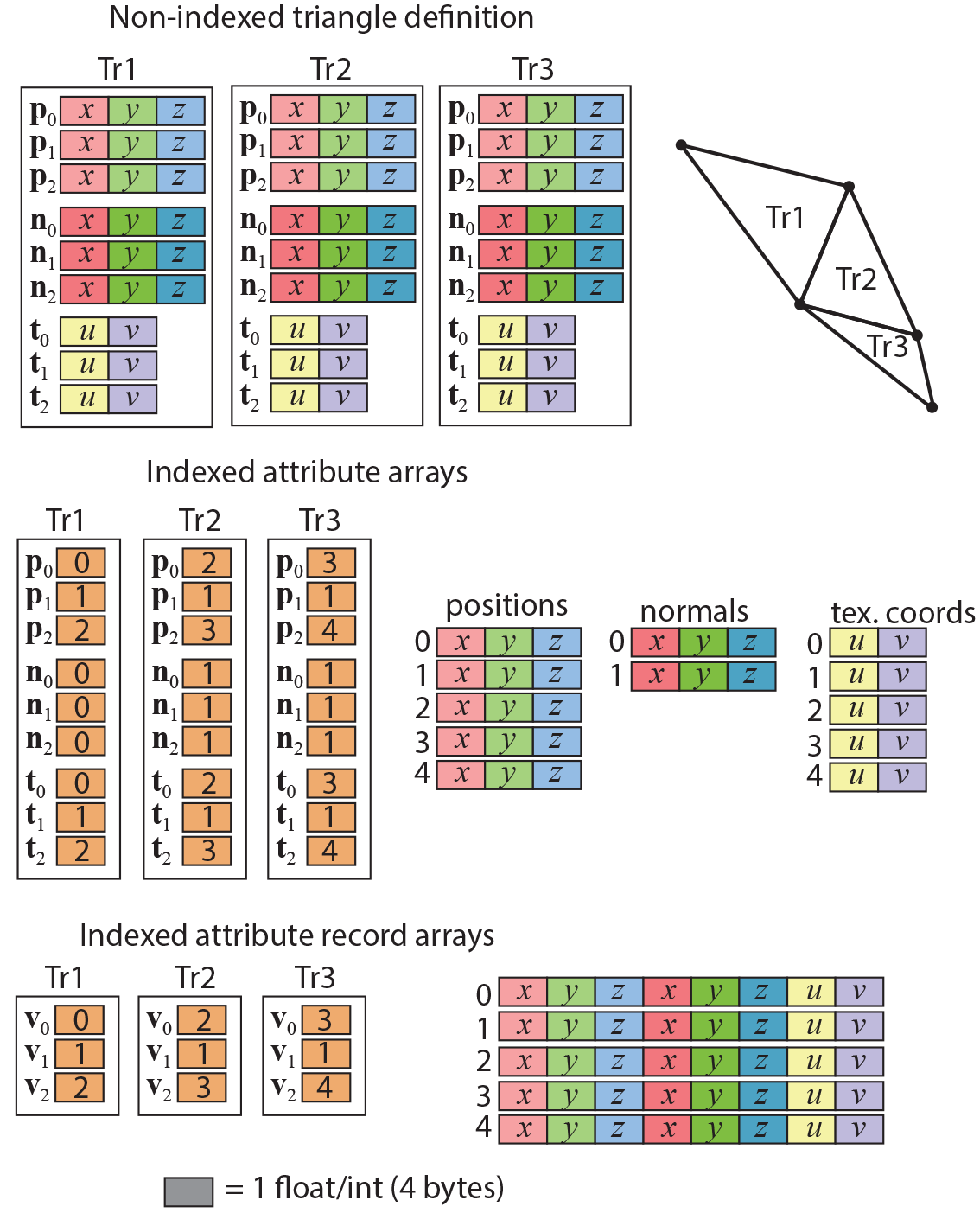
To access the vertex attributes of the corners of a triangle (or other polygon, for that matter), the polygon must either embed all the attribute data as part of the polygon representation (see first row in the following figure), or index separate arrays of vertex attribute data. In the former case, shared information is replicated, resulting in a quite wasteful representation. This is avoided in the case of an indexing scheme, where the polygon only maintains connections (indices) to records uniquely describing the (shared) vertex data. All polygons using a specific vertex, just index the same vertex attribute record.

Vertex information can be indexed in two different ways: create arrays of data for each different attribute and maintain a separate index per vertex for each one of the attributes, or create an array of attribute records and use a single index per vertex to indirectly access the entire record. Although the latter introduces some redundancy, when the same vertex has different auxiliary attributes for different polygons that use it, this is seldom the case and this configuration is more compact, especially for digitized assets.

Common Formats and Applications

Three-dimensional data are stored in numerous formats. However, there exist some widely used interchange formats that most mesh processing, 3D modeling, rendering and digitization software can export and import.

The Polygon File format (PLY), also known as the Stanford Triangle Format was initially designed for the storage of three-dimensional data from 3D scanners. The format is flexible enough to store from bare positional data of point clouds to indexed polygons and full per vertex information, including color, normal vectors and texture coordinates. There are two versions of the file format, one ASCII (hence human readable), the other binary. The PLY format is still being used for the interchange of 3D data, mainly due to its very simple structure and ability to customize and store per-vertex color (some other popular formats do not permit this). Most 3D acquisition software supports PLY as one of the output formats and mesh processing and 3D modeling software include import functionality for at least one version of it.

One of the oldest common formats around is the Wavefront Object format - OBJ. This is an ASCII file that can store polygons along with material properties specified per object. It also supports material maps for reflective properties and per-vertex normals (see example below). Many models found on the internet are saved in this format and almost every application that manipulates 3D shapes imports and exports files in OBJ form. Keep in mind that the OBJ format is modular, in the sense that the main file only contains the geometric information (objects, polygon groups, vertex attributes and connectivity). All material information is stored separately in an external file (.mtl extension). The same holds for texture images referenced from the material descriptions of the MTL file data. It is also important to note that the OBJ format does not support animation properties.

When objects that have been scanned and processed are intended for replication on a 3D printing device, these models must usually be "watertight", i.e. having an enclosing surface with no holes. A typical format for storing such data is the Stereolithography (STL) format. Despite the name, it has been extensively used for storing large 3D scanned meshes. It has both an ASCII and binary variant and only stores geometric information, without texture or color, hence its compact representation, which makes it ideal for very large datasets. 3D printing software and 3D scanning suites often include STL import/export functionality.

General 3D assets that are intended for use in interactive rendering applications involve a wider range of requirements. First of all, 3D models must support animation, either in the form of "keyframe" vertex animation (see relevant module) or as skeletal deformation animation. This implies that the target format must supply an extended set of description data for declaring dependencies, geometric transformations, vertex weights, motion control and interpolation methods, keyframes, etc. Another requirement that general 3D assets typically have is the ability to describe material properties of a diverse set of shading models used during rendering to properly compute lighting interactions with the surface and volume of the 3D shapes.

The two widely used formats in creative industries and applications for that purpose are the Filmbox (FBX) format and glTF (Graphics Library Transmission Format). These are commonly used for storing not only 3D models, but entire organizations of 3D objects (3D scenes), light setups, animations, materials and cameras. Being container formats, they are rather complex and extensive in their specification, but allow for greater descriptive freedom and support for application-specific information to be stored. FBX and glTF are mostly exported by modeling software and used in asset editing and manipulation tools, interactive rendering platforms and game engines as well as offline rendering pipelines.

Transformations

Geometric Transformations

The main operations that we perform on shapes in order to modify them and arrange them on the plane or in the three-dimensional space are called geometric transformations. For polygonal meshes and parametric surfaces, geometric transformations are applied to all vertex positions to modify an object as a whole, but in certain cases, they are also selectively applied only to specific vertices or vertex groups. When applying a geometric transformation, other vertex properties may be affected by it, such as the shading normal attached to a vertex. This makes sense, since a normal vector encodes a pointing direction for the underlying boundary (in 2D) or surface (in 3D), which is modified of the shape is rotated. The geometric transformations are always reversible, in the sense that we can always go back to the previous, pose and scale of an object, after applying a transformation to it, by applying the inverse transformation. For example, if we rotate a shape clockwise on the plane, we can always rotate it counterclockwise by the same angle to restore its original pose.

In a more general sense, geometric transformations create a spatial relationship between the reference frame local to a shape or part and its parent reference frame in terms of hierarchical dependency. For example, in the case of a 3D scene, a geometric transformation modifies the spatial relationship of the local reference frame of a newly added 3D asset, with respect to the global, top-level reference frame of the scene. Thinking in terms of relationships between dependent reference frames helps us generalize the concept to shapes that are not explicitly defined in terms of vertices and other entities that can be individually translated, rotated or scales themselves as constituent parts of a 2D/3D model.

Transformations on the Plane

On the 2D plane, the three basic transformations are translation, i.e. moving an object along a vector, rotation of a shape around the origin and scaling of its coordinates isotropically (uniformly) or with a different scaling factor in each dimension. The following figure illustrates these basic operations.

Transformations are represented mathematically in the form of matrices, which allows the easy application of a transformation to a vertex, but also facilitates the composition of multiple successive transformations into a single compound transformation (matrix). Each of the three elementary transformation matrices (translation, rotation, scaling) can be symbolically represented in a parametric form. Given a point $\mathbf{p}$ to be transformed, and the resulting point $\mathbf{p}'$, the notation for defining a geometric transformation is:

$$Translation: \mathbf{p}'=T_{t_x,t_y}(\mathbf{p}), \label{Eq:Transformations3}$$

$$Scaling: \mathbf{p}'=S_{s_x,s_y}(\mathbf{p}), \label{Eq:Transformations4}$$

$$Rotation: \mathbf{p}'=R_{\theta}(\mathbf{p}). \label{Eq:Transformations5}$$

In the above formulation of basic geometric transformations, each one has its own parameters; $t_x$ and $t_y$ represent the horizontal and vertical offset, when translating (moving) a shape. These can be considered as the coordinates of a vector that corresponds to the linear motion that affects the shape under translation (see example in the figure above). The parameter for the rotation is the angle of rotation (in degrees or radians) of the shape around the origin. For scaling, the parameters are the scaling factors $s_x$ and $s_y$ along the $X$ and $Y$ axis. Scaling factors represent ratios of the target over current scale of a shape in each direction. Values above 1 represent a magnification, while values lower than 1 and greater than 0 represent minification (shrinking). The two scaling factors should never be 0, because all coordinates of the shape would irreversibly collapse to 0 for the corresponding axis. Scaling factors can be identical, to enforce a uniform scaling, without any distortion.

Transformations are often composed to form larger sequences of operations, in order to perform more complex manipulations of shapes, for example:

$$\mathbf{p}'=T_{-1,2}(R_{45^o}(S_{\frac{1}{2},3}(\mathbf{p}))). \label{Eq:Transformations6}$$

In matrix, form the sequence of transformations is provided as a product of matrices applied (as a single matrix) to a vector/point. The above transformation composition can be written more compactly in matrix form as:

$$\mathbf{p}'=\mathbf{T}_{-1,2}\mathbf{R}_{45^o}\mathbf{S}_{\frac{1}{2},3}\mathbf{p}. \label{Eq:Transformations6}$$

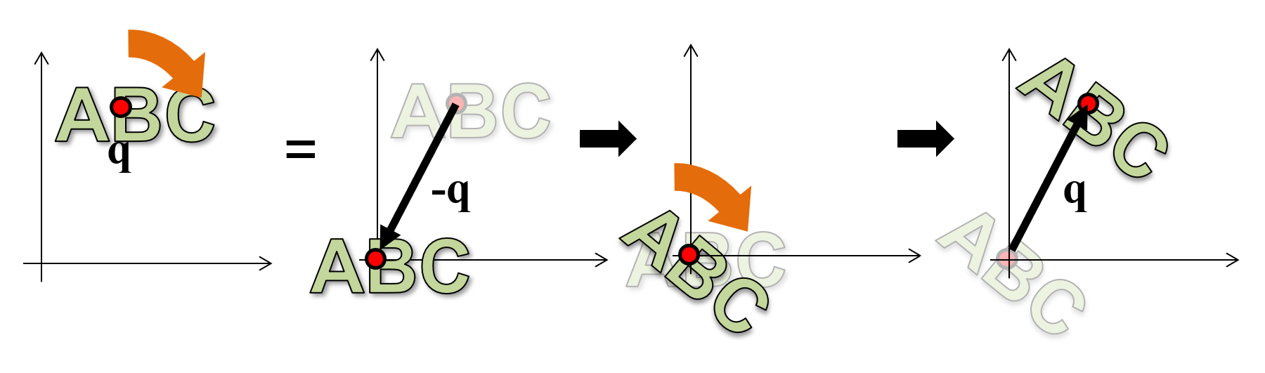
It is important to understand that both the rotation and the scaling transformations are applied with respect to the origin. There is no intrinsic notion of an arbitrary "pivot" point in the mathematical definition of these operations. When a shape is rotated, all of its vertices circle around point $(0,0)$. When a shape is scaled, its vertices move away from (magnification) or closer to (minification) point $(0,0)$. This is illustrated in the above figure. If we need to use an arbitrary pivot point $\mathbf{q}$ for the transformation, then we must first "make" the pivot point the origin and then perform the transformation. But how do we make an arbitrary point our temporary local coordinate system origin? Remember, transformations are all about creating spatial relationships among established coordinate systems (and their dependent data). So, we move the pivot point (and the shape) to the known reference system origin, perform the rotation or scaling and then, move back them back to the original location $\mathbf{q}$. This is in fact the dual transformation of moving the entire scene and the origin to $\mathbf{q}$ (so that now the origin rests at $\mathbf{q}$), performing the transformation and taking back the entire scene and coordinate system to where it was prior to the operation. The application of a transformation using a certain pivot point is demonstrated in the following figure.

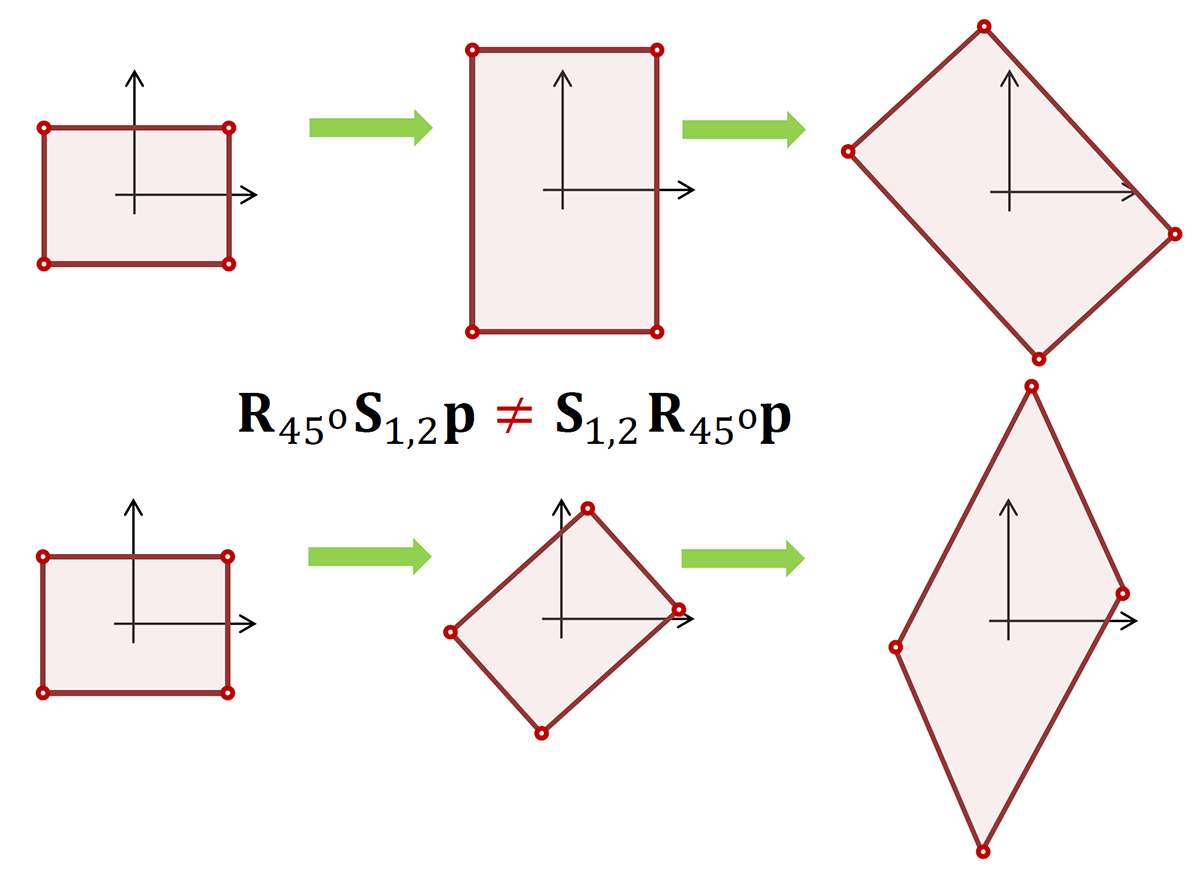
Please note that geometric transformations are not commutative, i.e. the sequence of the operations matters and changing it produces different results in general (see example in the next figure).

Transformations in 3D Space

Three-dimensional transformations follow a similar formulation to 2D ones, however, due to the increase in space dimensionality, translation offsets are now 3D vectors and scaling requires three factors instead of two. The following figures demonstrate the effect of the translation and scaling in 3D.

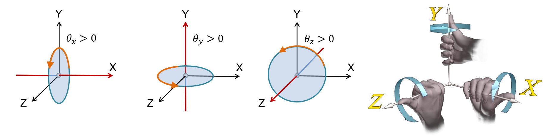
Elementary rotations are not restricted to a single plane, as in the two-dimensional case, and therefore an object can be rotated around any of three independent axes. In most practical cases, these rotations are defined around the primary axes of the coordinate system (rotations using Euler angles). The following figures demonstrate the effect of rotation around the $X$, $Y$ and $Z$ axes.

The corresponding operators become:

$$Translation:~ \mathbf{p}'=\mathbf{T}_{\mathbf{t}}=T_{t_x,t_y,t_z}(\mathbf{p}), \label{Eq:Transformations7}$$ $$Scaling:~ \mathbf{p}'=\mathbf{S}_{s_x,s_y,s_z}(\mathbf{p}), \label{Eq:Transformations8}$$ $$Rotation~around~axis~\mathbf{v}:~ \mathbf{p}'=\mathbf{R}_{\mathbf{v},\theta}(\mathbf{p}), \label{Eq:Transformations9}$$

Please note that rotations can be performed by a positive or a negative angle, determining a specific winding around the axis of rotation. When using a "right-handed" coordinate system, with the X axis point to the right, the Y axis pointing upwards and the Z axis extending backwards, positive rotations are given by a counter-clockwise rotation. To better get a grasp (literally here) of the correct positive rotation direction, you can align the thumb of your right hand with the positive axis direction and curl the rest of the fingers around the axis. This is the positive rotation direction, as demonstrated in the following figure. The opposite convention holds for the "left-handed" coordinate system.

Example: The following example demonstrates the use of geometric transformations to create a composite structure out of two given primitives, a cylinder and an arch brick. To build the intended shape (shown in red) we must use one instance of the arch and two instances of the cylinder. The two primitives do not initially lie on the origin, so we must be careful when applying geometric transformations to them; remember that the rotation and the scaling transformations are performed by definition with respect to the origin and not some arbitrary pivot point of our choice.

Let us start with the simplest case, that of the arch. According to the design, the arch’s final pose is perpendicular to the original positioning of the primitive and therefore a rotation by 90 degrees must take place at some point. A translation must be also occur so that the arch coincides with the final part’s position. However, we cannot yet surmise the exact X, Y and Z offsets, since the rotation is still pending and will alter the pose of the arch. Rotating the shape of the arch around the Y axis by 90 degrees, aligns the arch with the target part. Now we can measure the distance in each separate principal direction and concatenate the offsets along each axis in a single offset vector. Observing the footprint of the target arch part on the XY plane, we can see that there is no need to shift the position along the X axis, but the primitive must be moved 3 units towards the negative Z direction, i.e. by -3. Similarly, we can observe that the height of the columns the target arch C rests on is 2 units and presently the part lies on the XY plane, hence at Y $=$ 0. The arch must therefore be raised by 2 units, i.e. moved along the Y axis by 2. To sum up, the translation vector becomes: $\mathbf{t}=(t_x, t_y, t_z) = (0,2,-3)$. Putting the two transformations together we have:

$$\textrm{C}=\mathbf{T}_{(0,2,-3)}\mathbf{R}_{y,90^o}\textrm{Arch}. \label{Eq:transexample1}$$

The columns A and B are represented by a cylinder, but the axis of symmetry of the parts is parallel to Y whereas the primitive we are provided with has a cylinder axis parallel to axis Z. Clearly, we must rotate the cylinder but also change its size using a different scaling factor for the base and the height. Since the Cylinder primitive is positioned off-center with respect to the origin of the reference frame, performing the rotation and scaling at the original location of the Cylinder primitive will change the position of the cylinder, at the same time. This can hinder our ability to easily calculate the required offsets for the final placement of parts A and B. To address this, we can first translate the cylinder so that the intended pivot point rests on the axis of rotation (X here). We can also arrange for the base of the cylinder to be symmetrically positioned across one axis of the intended base of the column (here Z, or Y), although we could alternatively make the cylinder touch the XZ plane with one side. During scaling, coordinates move away or towards the origin of the coordinate system and with either of the suggested offsets along the X axis, we can predictably alter the dimensions of the base of the cylinder. The proposed translation is $\mathbf{T}_(4,0,-1)$. Again other convenient offsets could be provided to facilitate rotation and scaling, such as $\mathbf{T}_(4,-1,-1)$ (you can try this as an exercise, to see how the subsequent transformations provided below are affected).

Next, we can perform the rotation of the cylinder and the change of scale so that the column takes up the right proportions and orientation. However, one can observe that the specific order of operations is not crucial, since there exist appropriate scaling and rotation transformations to obtain the same result, albeit with order-dependent, different parameters. Assuming a rotation followed by scaling, we must first rotate Cylinder around the X axis by -90 degrees (clockwise in a counter-clockwise coordinate system) to align the base with the XZ plane. Then a scaling of the base by a factor of $0.5$ must be performed (along both X and Y directions), combined with a height extension by a factor of 2. The resulting scaling operation is $\mathbf{S}_(0.5,2,0.5)$. Combining the transformations so far we get:

$$\mathbf{M}_{column}=\mathbf{S}_{(0.5,2,0.5)}\mathbf{R}_{x,-90^o}\mathbf{T}_{(4,0,-1)}. \label{Eq:transexample2}$$

Alternatively, if we have chosen to perform a scaling first, followed by a rotation, the corresponding transformations would have been: $\mathbf{S}_{(0.5,0.5,2)}$ followed by $\mathbf{R}_{x,-90^o}$.

Finally, to create part A, a translation by $(0.5, 0, -1)$ is required:

$$\textrm{A}= \mathbf{T}_{(0.5, 0, -1)}\mathbf{M}_{column}\textrm{Cylinder}=\mathbf{T}_{(0.5, 0, -1)}\mathbf{S}_{(0.5,2,0.5)}\mathbf{R}_{x,-90^o}\mathbf{T}_{(4,0,-1)}\textrm{Cylinder}. \label{Eq:transexample3}$$

Notice that part B is the same as part A but with a slightly different final offset. To create it, we use a second instance of the cylinder, apply the same transformation up to the final translation and apply a translation by $(2.5, 0, -1)$ instead of $(0.5, 0, -1)$:

$$\textrm{B}= \mathbf{T}_{(2.5, 0, -1)}\mathbf{M}_{column}\textrm{Cylinder}=\mathbf{T}_{(2.5, 0, -1)}\mathbf{S}_{(0.5,2,0.5)}\mathbf{R}_{x,-90^o}\mathbf{T}_{(4,0,-1)}\textrm{Cylinder}. \label{Eq:transexample3}$$

Cameras

Viewing Transformation

The pose of cameras is defined in the coordinate system of the virtual scene (WCS) in the same manner as other objects, i.e. via some geometric transformation. What is special about a camera object is that it typically makes no sense to change the scale of the camera or a virtual eye, since the field of view of a camera is controlled by other, internal parameters (see next). This leaves only rotations and translations as meaningful geometric transformations to be applied to a camera system. These comprise the set of rigid transformations, also known as roto-translations, i.e. transformations that do not affect the shape of the geometry they are applied on.

Camera transformations are important because they position the virtual observer inside the virtual environment and keep doing so, during any interactive update to the viewpoint, either directly or indirectly via the transformation of an entity the camera is attached on. The rigid transformation of the camera defines its position and orientation and therefore the relation of its local coordinate reference frame with respect to the global coordinate system. Conversely, if we are provided with the inverse transformation, we can use it to express the coordinates of objects in the WCS in the eye coordinate system (ECS), which is the egocentric, local coordinate system of the camera. Depending on the underlying rendering architecture, the sampling process of a rendering algorithm may occur after transformation of geometry to either ECS (rasterization) or directly in WCS (e.g. ray tracing).

To better understand the duality of the relative transformations, lets examine the following example: We have a camera pointing towards the negative Z axis that is translated towards the left (-X) by some offset $d$. If we are a fixed observer with respect to the WCS of the scene, we will register the motion as a translation by a vector $(-d,0,0)$. Now what does the camera see? If we observe the world "through the eye" of the virtual camera, we consider this egocentric reference frame, the ECS, as our anchor and perceive the relative motion of everything else with respect ot the camera. This means that by shifting the camera to the left, we experience the world being shifted to te right, as we observe it moving along with the camera. So we perceive the world being translated by $(d,0,0)$, i.e. $d$ units towards the positive X axis. However, this is the inverse transformation of the rigid motion applied to the camera, since the inverse of a translation by some vector, is the translation by the opposite vector.

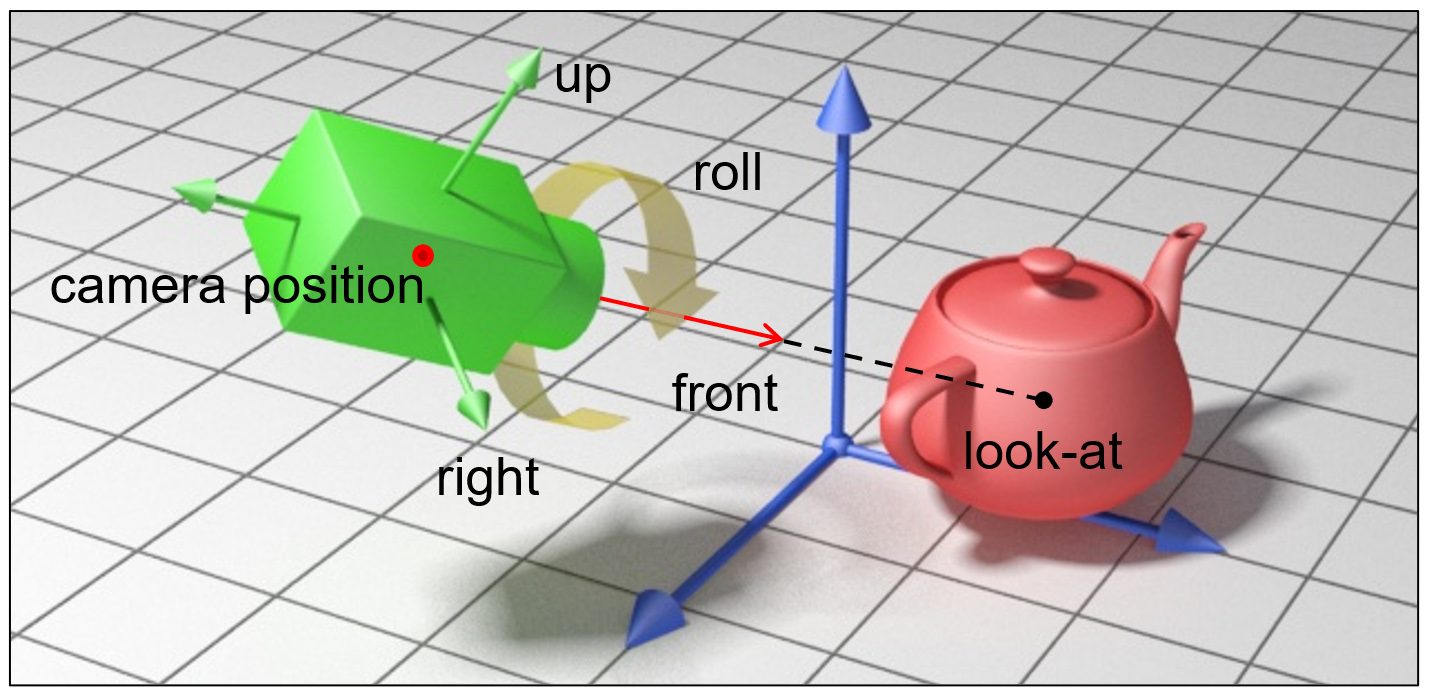
The camera transformation can be given directly by supplying a sequence of rotations and translations or indirectly by computing the rigid motion from the supplied vectors of the local coordinate system of the camera and its position. In many cases, this is preferable, as we can more intuitively manipulate and define the local coordinate system of the camera. For instance, specifying the "gaze direction" or "look at" vector of a camera, essentially translates to specifying the -Z axis of the ECS.

But why is it important to be able to express the coordinates of the world with respect to the eye coordinate system? The popular rendering pipeline of rasterization, which is nowadays implemented in the hardware of the graphics processing units and has prevailed as the most efficient image generation approach for more than 40 years, performs image synthesis by sampling primitives in image space, after first transforming and projecting them in eye space. Moving all coordinates to eye space prior to projection and sampling, vastly simplifies computations and comparisons, since the local Z camera axis acts as a natural depth sorting direction of coordinates being closer or further away from the center of projection. Other operations, such as perspective division (see next) and clipping, are also simpler to perform, when the perceived depth direction is aligned with a major axis (Z).

Projections

In computer graphics, a projection is the process and respective mathematical operation that maps a three-dimensional shape onto a two-dimensional parametric surface, typically to form an image. We are usually concerned with projections from 3D space to a plane, called the plane of projection, although other surfaces are also of interest, such as spherical, hemispherical, or cylindrical, which are used in specific applications and display systems.

Two projection families are commonly of interest:

• Parallel projection, where the distance of an imaginary center of projection from the plane of projection is infinite;

• Perspective projection, where the distance of the center of projection from the plane of projection is finite.

Parallel Projection

In a parallel projection, the (imaginary) center of projection is considered to be at an infinite distance from the plane of projection and the "projector lines", i.e. the lines connecting the three-dimensional coordinates and their projection on the plane, are therefore parallel to each other. To describe such a projection one must specify the direction of projection (a vector) and the plane of projection. We may distinguish between two types of parallel projections: orthographic, where the direction of projection is perpendicular to the plane of projection, and oblique, otherwise. Keep in mind though that oblique projections can be obtained by first applying a sequence of elementary geometric transformations prior to performing an orthographic projection.

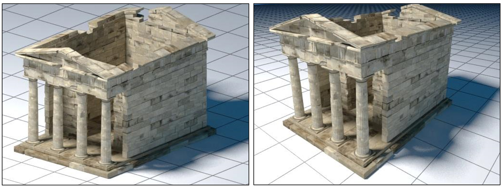
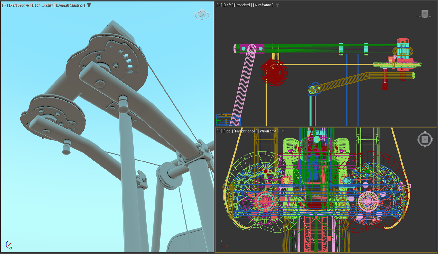
Parallel projections are important to graphics and particularly 3D modeling and computer-aided design, because they provide a visualization of a 3D model, where relative angles and distances are preserved across the projection plane; the projections of two line segments of equal length, are always equal. Also equal angles between two vectors in 3D space correspond to equal angles between the projected vectors. This makes measuring distances and making comparisons possible, during the design of 3D assets. Therefore, it is pretty common to utilize (multiple) planar views of the design space, where actual drawing of elements, geometric transformations and modeling operations are performed.

Perspective Projection

Perspective projection. The perspective projection transformation "flattens" a shape on an image plane and being a non-linear one, distorts the relative distances of object coordinates (perspective foreshortening) and in general, also alters the angle between lines. Our eyes, along with most imaging devices, follow similar principles and therefore, produce a similar perspective distortion. Practical sensors also introduce many types of spherical distortion, which further bend the captured image. In computer vision, the perspective projection parameters along with other distortion factors are collectively known as intrinsic camera parameters. In order for a digitization system to correctly recover the shape of perceived geometry registered in the sensor’s image plane, all the factors and parameters that contribute to the projection’s distortion must be known (or learned) beforehand.

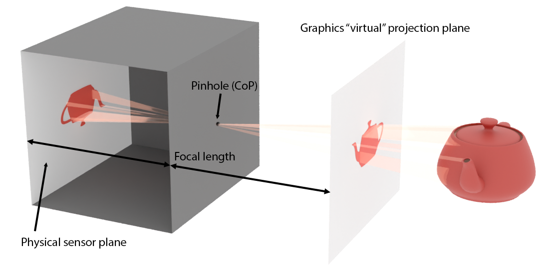
In computer graphics, the simplest perspective projection modeling considers an idealized camera system, the pinhole camera model. This model attempts to simplify computations and mathematics involved in the generation of an image and thus dispenses with the physically-accurate modeling of real camera systems. The model assumes that light passes through a tiny opening, a "pinhole", which acts as the center of projection. The image plane in a physically plausible construction would lie at the back side of the imaging device, at a distance called the focal length. However, the projection formed on the "sensor" of a real camera system would be inverted, as shown in the figure that follows. In mathematics and in computer graphics by extent, we can virtually and symmetrically move the projection plane a distance equal to the focal length in front of the center of projection (pinhole) so that the image on the plane is not inverted any more.

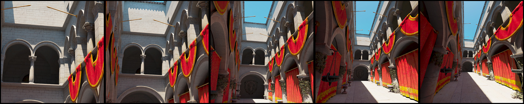
The relative height and width of the image plane extents over the focal length determine the angular opening of the camera. Assuming a fixed image plane, a shorter focal length would correspond to a wider field of view, whereas a long focal length would mean the modeled camera is a tele-photo device. A large focal length introduces less perspective foreshortening distortion than a short one. This is demonstrated in the following figure.

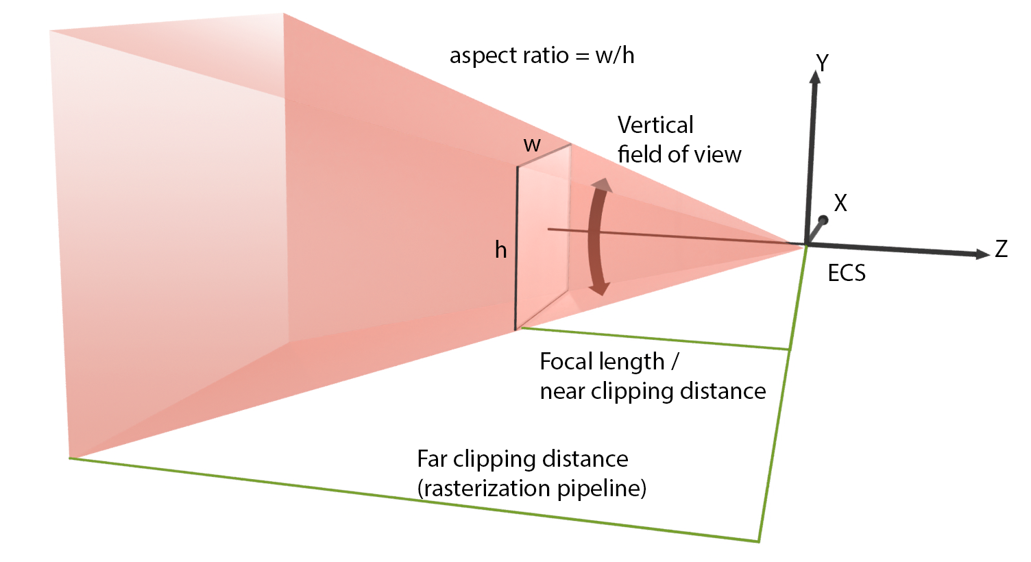
In practical terms, to set up a perspective projection camera, one must either provide the extents of the projection plane window ($w, h$ in the next figure) and the focal length or, more conveniently, directly set the field of view angle. Since the image projection rectangle is not square in general, we provide either the horizontal or the vertical field of view aperture, and the aspect ratio of the imaging window. The latter is usually automatically determined by the respective aspect ratio of the synthesized image resolution.

In real-time graphics that use the rasterization pipeline, it is essential to provide both a minimum clipping distance and a maximum one. That minimum (near) clipping distance, which corresponds to the distance of the projection plane from the center of projection of the resulting camera, is compulsory for the derivation of the mathematical representation of the projection matrix. The maximum (far) clipping distance limits the visible geometry and maximizes the representation accuracy important in the hidden surface determination algorithm (see Rendering unit). Clipping very distant geometry is a good practice to avoid submitting too many polygons of the virtual environment for rendering. This is especially important for large, open virtual environments. The visualization of very distant objects is often replaced by proxy geometry (at a closer distance) or the display of a surrounding image panorama (an environment map) as the background of the view. Special effects, such as fog or atmospheric attenuation, are also employed to mask the transition to the "distant" environment.

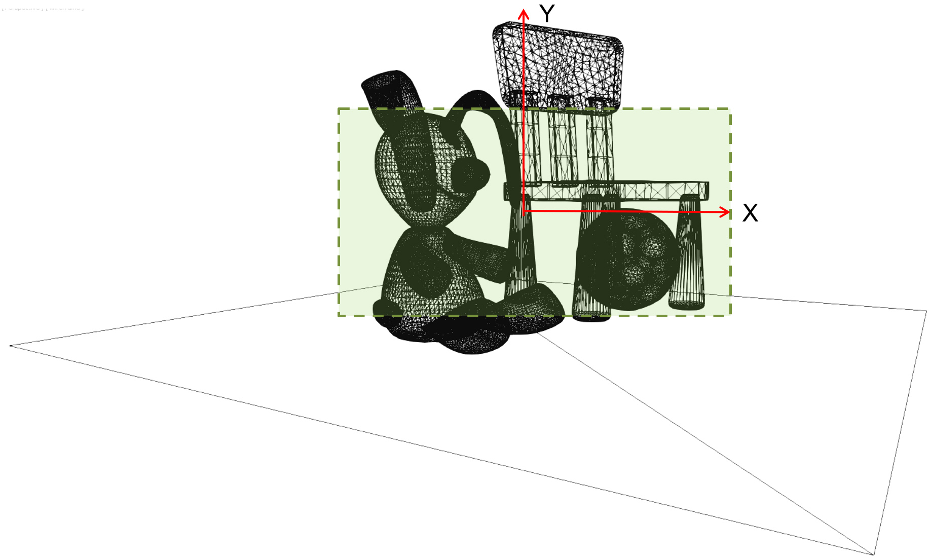
Bounding Volumes

An Overview of bounding Volumes

Every 2D and 3D shape can be fully enclosed in another, simpler and most importantly, convex shape of appropriate dimensions. In the two-dimensional case, such a shape can be a circle or a quadrilateral. In three dimensions, simple primitives such as spheres, boxes or other slab-like shapes can serve as such enclosing surfaces. Although the case of 2D graphics is also important, we shall focus here in three dimensions, where bounding volumes play a very important role in making complex computations practical.

A bounding volume is typically used as a proxy to the contained group of primitives to quickly test the overlap of the group with a given interval in 2D or 3D space or another set of primitives. Such an operation arises extremely often in ray tracing and collision detection for animation. For example, a ray is tested for intersection first with the container (the bounding volume) and if the test is successful, i.e. the ray passes through the bounding volume, then and only then are the contained primitives examined. This saves many computations, in the case that the ray does not overlap with the container. The same acceleration scheme is applied to collision detection. Very often, collision, i.e. spatial overlap between two objects each made of a set of primitives, is done between proxy bounding volumes. In many cases, and if the bounding volumes are good approximations of the original object shapes, the collision testing stops there and an approximate result is returned. If more accuracy is desired, the collision system may go inside the bounding volumes and examine detailed primitive intersections between the two sets of primitives.

There are two important factors when choosing a bounding volume for a shape, which often contradict one another:

• Tightness. If a bounding volume fits loosely on the contained geometry or the vacant space left due to the shape having many protruding parts or being inconveniently posed is large, the bounding scheme is sub-optimal and inefficient. The larger the bounding volume is with respect to the actual volume of the enclosed structure, the worse the performance of the bounding volume is as a proxy for the object; if the bounding volume leaves too much void space, the probability of false positive intersections with it grows. Too many intersections with the bounding volume will be reported that will lead to a wasteful and failed detailed search for intersection with the contents. The role of a bounding volume is to minimize the number of times its contents are queried or an operation with them is triggered.

• Complexity. Since the intent of using a bounding volume is to delegate most of the overlap tests with its own geometry instead of its contents, the calculations involved must be kept to a minimum. This is why simple geometric shapes with easy overlap tests are often favored, despite them not being optimal in terms of tightness.

Common 3D Bounding Volumes

The most cost-effective to compute intersections with and thus the most commonly used bounding volumes for generic aggregations of primitives are the sphere and the box (orthogonal parallelepiped). Spheres are very useful for testing collisions with other spheres, since the test boils down to checking whether the distance between the two sphere centers is smaller or equal to the sum of their radii. Spheres are therefore a favorite BV for collision detection systems. Spheres can be also grouped and hierarchically organized (although not as efficiently in terms of tightness as boxes) to form sphere trees, which help provide an affordable means to compute relatively precise collisions among elaborate objects.

Still, the most generic and widely used primitive in computer graphics for the representation of a bounding volume is the axes-aligned bounding box, or AABB. Axes-aligned means that its sides in 2D are parallel to the primary axes (X, and Y), while in 3D they are parallel to the primary projection planes (XY, YZ, ZX). This greatly simplifies interval testing calculations, making the line-box and box-box overlap computations very efficient. AABBs are used for a wide range of applications, from collision detection and visibility testing to ray tracing and geometry processing. An axes-aligned bounding box is also simple to represent and calculate for an aggregation of primitives: it is defined by the minimum and maximum extents of the primitive cluster in each axis, i.e. the minimum and maximum X, Y and Z coordinate. Alternatively, one can set up an AABB by defining its center and a vector of scaling factors for each axis (assuming an initial unit-sized cube). Because of this simple definition, it is also efficient to cluster AABBs to form aggregations and hierarchies: the extents of an AABB containing other AABBs are simply the minimum and maximum extents of its contents ("children" AABBs). AABBs are therefore the favorite primitive for building bounding volume hierarchies (BVH) ³.

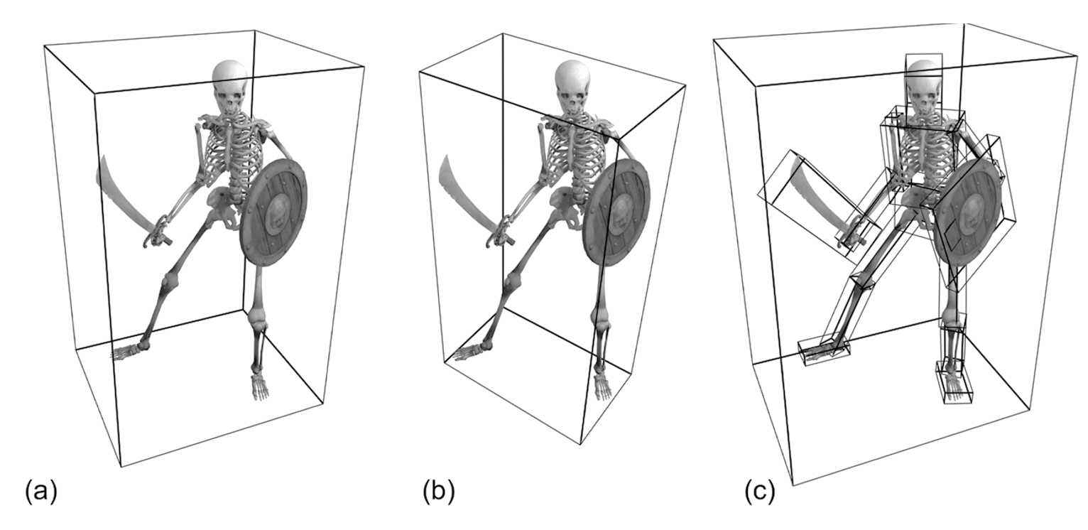
Axes-aligned bounding boxes constitute a very compelling option for a spatial container, mainly due to their efficient construction and overlap testing. However, they are invariably not the most tightly-fitting shapes, with same extreme cases being notoriously inefficient in terms of spatial coverage, such as the bounding of a long and thin structure diagonally positioned with respect to the primary axes. To counter this problem, a logical alternative is to re-orient a box so that it better fits the underlying collection of primitives in terms of residual void space (tightness). This BV is called an oriented bounding box (OBB). The OBB is still an orthogonal parallelepiped, but not aligned with the primary axes any more. The box uses a local coordinate system different from the global one, which is calculated based on the spatial distribution characteristics of the contained primitives. This calculation, although not very complex itself, is generally not as efficient as computing the extents of an AABB. The alignment of the box with an arbitrary coordinate system also implies that testing for overlap with lines and other structures is a bit more convoluted: An OBB is in essence an AABB when expressed in its own, local reference system. Checking for intersections with an OBB therefore requires applying a geometric transformation to go from one coordinate system to the local coordinate system of the OBB and then perform the intersection test with the OBB treated as an AABB with respect to its local coordinate system. IF the intersection results are important for the task at hand, e.g. an intersection point, then the locally computed result must also be transformed back to the coordinate system we operate on.

To summarize, AABBs offer very fast construction and overlap testing performance but lack in terms of tightness, making them more susceptible to wasteful false positive tests. OBBs on the other hand are quite the opposite: they offer very good tightness but construction and intersection times are increased compared to the AABBs.

Regardless of the tightness or intersection performance of any of the bounding volume shapes suggested so far (there are indeed other options investigated in the bibliography, such as k-DOPs, bounding capsules, etc.), there are two other important problems to address, when attempting to create proxies for overlap testing with a group of primitives:

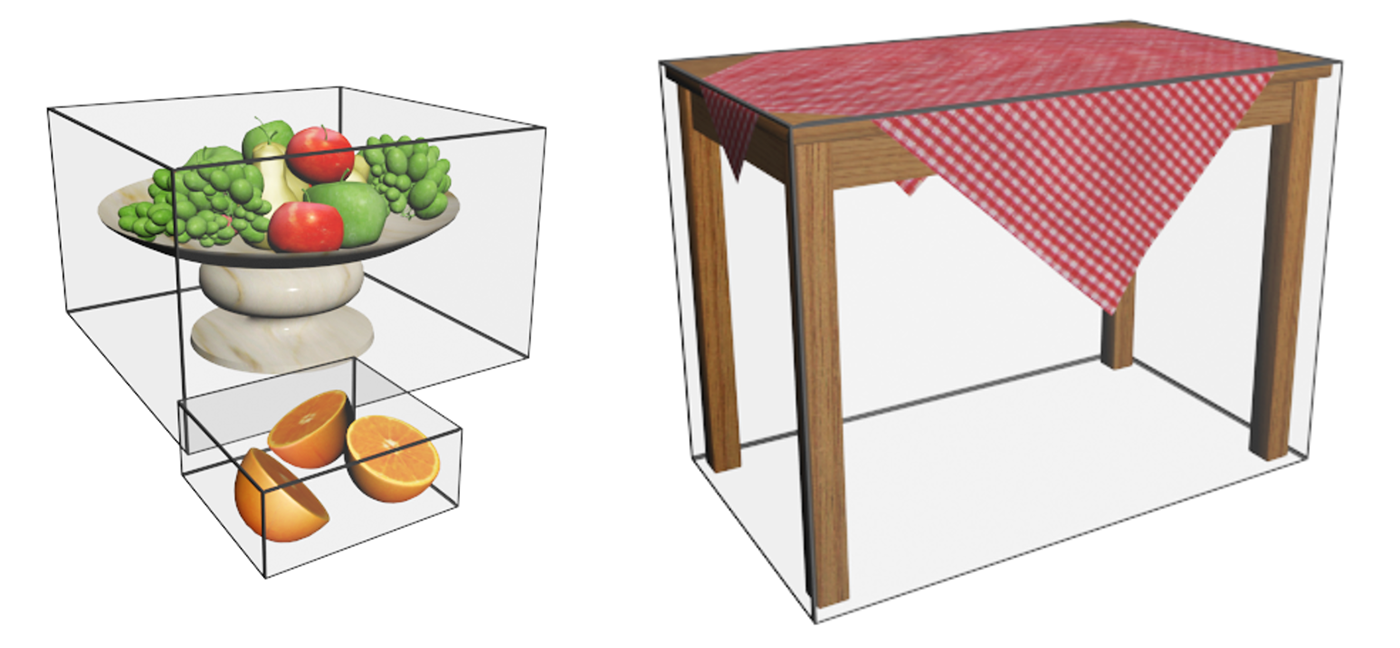
• The shape of the enclosed primitive cluster. Shapes with protrusions and elongated parts, large cavities or disjoint sets of primitives will invariably leave too much void space between the bounding volume and the enclosed geometry (see the table in the first example or the figure below), no matter what the choice of a bounding volume is.

• The number of enclosed primitives. When a positive overlap is detected with the bounding volume, we frequently require that a detailed intersection is reported with the contained geometry (if any). If the number of contained primitives within the BV is large, exhaustively testing each one of them for intersection is very inefficient.

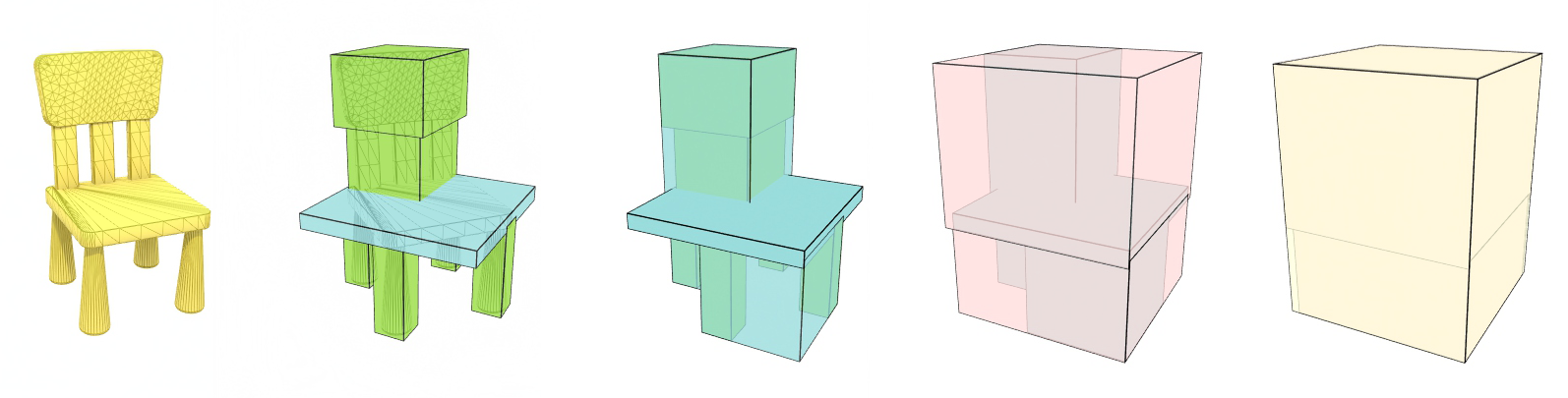
To solve both problems, in computer graphics we resort to hierarchically arranging bounding volumes, organizing primitive clusters in as small and spatially coherent groups as possible and nesting them within bounding volume hierarchies (BVH). BVHs depend on the spatial locality of contained elements at each hierarchy level in order to ensure tight fitting, regardless of the bounding primitive used (which is usually an AABB, but not always). Furthermore, spreading the actual geometric primitives across multiple "leaf" (bottom-level) nodes of the hierarchy, ensures that no single bounding volume contains a large number of geometric primitives, thus keeping the exhaustive overlap checks bounded and manageable. The larger the initial population of geometric primitives is, the higher the hierarchy becomes, respecting a maximum leaf-node population. However, traversing a hierarchical structure has a sub-linear cost compared to just organizing geometric primitives in a flat collection of bins. Binary trees are a common choice for constructing a BVH, but wider trees are also used in many applications, to further shorten the hierarchy at the expense of a more complicated building strategy and traversal stepping.

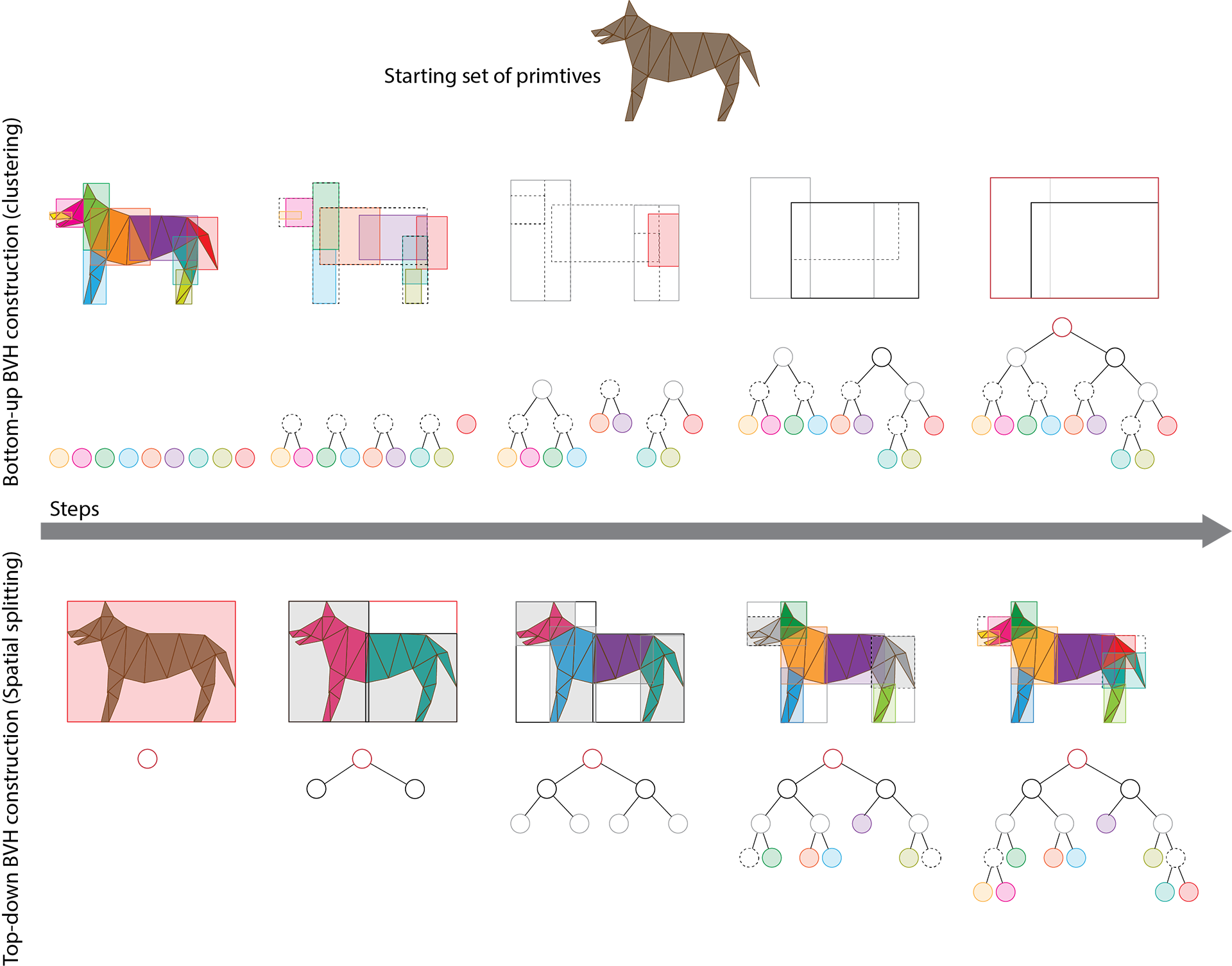
Bounding volume hierarchies can be built in two different ways: bottom-up or top-down. In the first case, the building method attempts to quickly cluster primitives based on their spatial location and then keeps aggregating the resulting bounding volumes to form larger container BVs. The process stops when all aggregate BV nodes are clustered in a single bounding volume for the entire object. Needless to say, the "object" can be an entire virtual world.

The second strategy starts by subdividing the space occupied by the entire geometry into strata, distributing primitives in each sub-container. The process is recursively repeated until a desired cost limit is reached. The cost typically involves the number of primitives at the leaf nodes and the shape of the resulting bounding volume domains. The algorithm attempts to minimize at the same time the tree depth, the number of primitives per leaf node and the residual space. For polygonal primitives, a spatial subdivision hierarchy results in a potentially overlapping set of sibling BVs (unless primitives are split at the boundaries of BVs). However, for point clouds, this strategy inherently leads to non-overlapping sub-volumes, making the search for intersections with the spatial hierarchy more efficient. After splitting a BV in sub-domains, each sub-volume can be shrunk to a tight bounding volume before splitting it further.

References

---

1. Image created by Philip Tregoning, Public Domain, https://commons.wikimedia.org/w/index.php?curid=1099269↩︎

2. In other rendering pipelines, too, depending on the modeling of the camera.↩︎

3. Although not necessarily the most efficient in terms of tightness and general performance, see (Vitsas et al. 2023)↩︎